Learning-based Distance Evaluation in Robot Vision
A Comparison of ANFIS, MLP, SVR and Bilinear Interpolation Models
Hossam Fraihat, Kurosh Madani and Christophe Sabourin
I LISSI / EA 3956 Lab., University Paris-Est Creteil, Senart-FB Institute of Technology,
36-37 Rue Charpak, 77127 Lieusaint, France
Keywords: Visual Distance Evaluation, Soft-Computing, Kinect, Visual Information Processing, Machine Learning,
ANFIS, MLP, SVR, Bilinear Interpolation.
Abstract: This paper deals with visual evaluation of object distances using Soft-Computing based approaches and
pseudo-3D standard low-cost sensor, namely the Kinect. The investigated technique points toward robots’
vision and visual metrology of the robot’s surrounding environment. The objective is providing the robot
the ability of evaluating distances between objects in its surrounding environment. In fact, although
presenting appealing advantages, the Kinect has not been designed for metrological aims. The investigated
approach offers the possibility to use this low-cost pseudo-3D sensor for distance evaluation avoiding 3D
feature extraction and thus exploiting the simplicity of only 2D image’ processing. Experimental results
show the viability of the proposed approach and provide comparison between different machine learning
techniques as Adaptive-network-based fuzzy inference (ANFIS), Multi-layer Perceptron (MLP), Support
vector regression (SVR), Bilinear interpolation.
1 INTRODUCTION - PROBLEM
POSITION
Robots’ visual perception of their surrounding
environment and their ability of metrological
information extraction from the perceived
environment are the most important requirements for
reaching or increasing robots’ autonomy (for
example for autonomous navigation or localization)
within the environment in which they evolve
(Hoffmann, 2005). However, the complexity of real-
world environment and real-time processing
constraints inherent to the robotics field make the
above-mentioned tasks challenging. In fact, if the
use of sophisticated vision systems (e.g. high-
precision visual sensors, sophisticated stereovision
apparatuses) combined with sophisticated processing
techniques may offer an issue for overcoming a
number of the above-mentioned requirements within
the condition of quite slow dynamics, they remain
either too expensive for every-day applications or
out of real-time processing ability for prevailing
dynamics inherent to the concerned field.
The recent decade has been a token of numerous
progresses in computer vision techniques and visual
sensors offering appealing potential to look at the
above-mentioned dilemma within innovative slants.
In fact, on the one hand, numerous image processing
techniques with reduced computational complexity
have been designed and on the other hand, a number
of new combined visual sensors with appealing
features and accessible prices have been presented as
standard market products. “Kinect”, a Microsoft
product which has been initially designed for Xbox
play station in 2008, is a typical example of such
combined low-priced standard-market visual sensor
that allows a pseudo-3-D visual capture of the
surrounding environment by providing the depth (in
meters) using an infra-red device and an color image
using a standard camera (Borenstein, 2012).These
depth and color image are subjected to a Soft-
Computing based approach hybridizing conventional
image processing in order to extract the estimated
distance between the objects.
It a previously realized work, we have
investigated an Adaptive Neuro-Fuzzy Inference
System (ANFIS) approach and its comparison with a
geometric method using the Kinect (Fraihat et al.,
2015).
The rest of this paper is organized as follows: In
section 2 a brief overview of our approach for the
168
Fraihat, H., Madani, K. and Sabourin, C..
Learning-based Distance Evaluation in Robot Vision - A Comparison of ANFIS, MLP, SVR and Bilinear Interpolation Models.
In Proceedings of the 7th International Joint Conference on Computational Intelligence (IJCCI 2015) - Volume 3: NCTA, pages 168-173
ISBN: 978-989-758-157-1
Copyright
c
2015 by SCITEPRESS – Science and Technology Publications, Lda. All rights reserved
estimation of the distance between objects. Section 3
introduces the proposed approach. Section 4 presents
the Experiments and Results. Finally, discussion and
conclusion in Section 5.
2 PROPOSED A
SOFT-COMPUTING BASED
APPROACH
The investigated approach, based on the Soft-
Computing techniques and the conventional image
processing of 2-D color image and depth
information provided by the Kinect, consists of three
phases (see Fig 1):
1. Capturing 2-D color and depth images from
Kinect.
2. Conventional processing of the Kinect issued
images extracting appropriate features.
3. Learning the extracted features (in learning
mode) or estimation of distance between
objects (in generalization mode).
Phase1: Capturing 2-D color and depth images from
Kinect.
The Kinect sensor can capture 2D color images
at a resolution of up to 640-by-480 pixels at 30
frames per second. The depth data image contain the
distance, in millimeters, to the nearest object at that
particular (x, y) coordinate in the depth sensor's field
of view. The Kinect can provide the depth image in
3 different resolutions: 640x480 (the default),
320x240, and 80x60 (see Figure2).
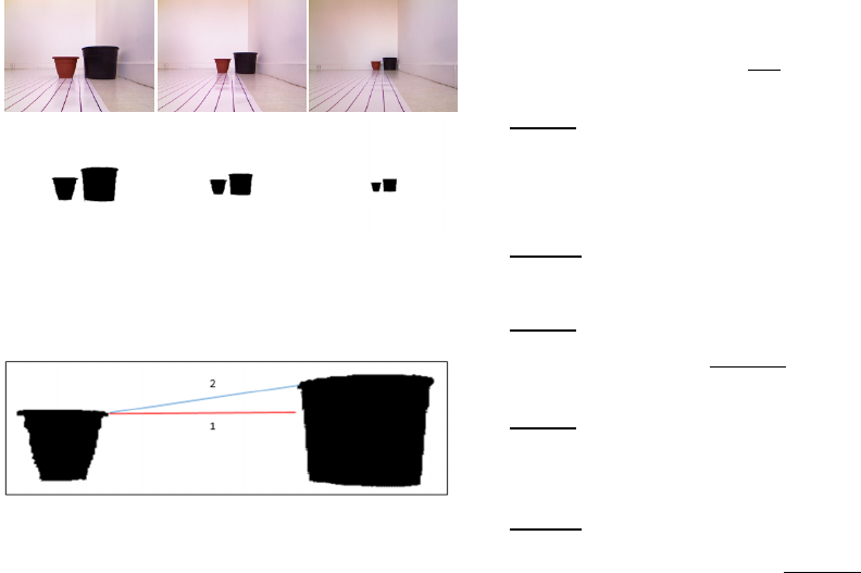
Figure 1: Block diagram of the proposed approach:
Learning Mode (upper) and Generalization Mode (lower).
Figure 2: The 2-D color and depth images captured by
Kinect.
Phase2: Conventional processing of the Kinect
issued images extracting appropriate features.
The Phase 2 consist of several Pre-processing
steps. It concerns the processing of data provided by
Kinect’s sensors. The visual data (namely the color
image) is segmented and a resulting binary image is
constructed. The considered techniques are
conventional segmentation techniques which have
been chosen on the basis the low-computational
complexity in order to fit real-time computation
constraints (Gonzalez and Woods, 2004). However,
more sophisticated processing techniques may be
used as those proposed by (Moreno et al., 2012).
Our approach used the mean shift segmentation
method, (Kheng, 2011) (Comaniciu and Meer,
2002), (Comaniciu et al., 2000).
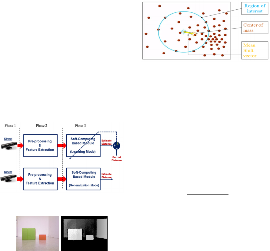
Figure 3: The principle of the mean shift segmentation
method.
The mainly task of the mean shift method is to
estimate the exact mean location “m(x)” of the data
(center of mass in Fig.3) by determining the shift
vector from the initial mean(region of interest in
Fig.3), the process will be repeated until find the
center of the region that represents maximum
density of pixels. Mean shift vector follow the
direction of the maximum increase in the density. To
calculate the mean location m(x) at the point x, we
use the equation (1), where n represent the number
of point in the kernel K of the region of interest,
x
is data point, x initial mean location and K
x
)
stands
for kernel function relative to the samples x
contributing to the estimation of the mean location.
)
∑
K
xx
)
x
∑
K
xx
)
(1)
The mean shift is the difference between m(x) and x,
it is an iteratively algorithm, stops when
)
. It is computed iteratively for obtaining
the maximum density in the local neighbourhood.
Mean shift has the direction of the gradient of the
density estimate. The gradient of the density
estimate give as how many pixels similar and
neighbour in a kernel. Fig.4 shows the results of
Learning-based Distance Evaluation in Robot Vision - A Comparison of ANFIS, MLP, SVR and Bilinear Interpolation Models
169
application of the mean shift segmentation method
on a set of different images. These images provided
by Kinect for a same distance of two given objects
captured close, farther and far from the Kinect. Once
segmentation is performed, the minimum distance
between the objects is calculated (number of pixels).
Such distance is defined as the minimum distance
between two horizontal pixels in each object (line 1
in Fig.5).
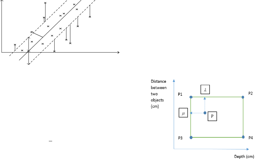
Figure 4: Example of captured images for two given
objects located at the same distance from each other. The
second row gives the pre-processed results of those
images.
Figure 5: The line1 represent the minimum distance
between two objects.
Phase3: Learning the extracted features (in learning
mode) or estimation of distance between objects (in
generalization mode).
The Soft-Computing based module estimates the
distance accordingly to different learning machine.
In the next section we present the different Learning
Machine used in our approach to estimate the real
distance in centimetre between the different objects.
3 BRIEF OVERVIEW OF USED
SOFT-COMPUTING MODELS
3.1 ANFIS
ANFIS is a Fuzzy Inference System (FIS) and using
Artificial Neural Network (Jyh-shing Roger Jang et
al., 1995) (Jang et al., 1997). The rule base contains
two fuzzy rules of Takagi and Sugeno’s type (Jyh-
shing Roger Jang, 1993) , expressed here-bellow,
where , are two input data,
is the Fuzzy
inference according to the desired output,
,
are
labels of fuzzy sets characterized by appropriate
membership function.
:
,
:
,
The membership functions of
, denoted
μ
x
)
, are given by equation (2), where
,
is the parameters set.
μ
x)
)
(2)
Layer1: Generating degree of membership, where
,
is the node function, where k is the number of
the layer and i is the node position in the layer.
,
μ
)
, 1,2
Layer 2: Fuzzy intersection.
,
μ
)
.μ
)
, 1,2
Layer3: Normalization.
,
1,2
Layer4: Defuzzyfication, where
,
,
is the
parameters set (consequent parameters).
,
)
Layer 5: The final output
,
∑
∑
3.2 Multi-Layer Perceptron (MLP)
Section
The Multi-Layer Perceptron (MLP) (Rumelhart et
al., 1986) (Lippman, 1987) is a very well known
artificial neural network organized in layers and
where information travels in one direction, from the
input layer to the output layer.
The input layer represents a virtual layer associated
to the inputs of data. It contains no neuron. The
following hidden layers are layers of neurons. The
outputs of the neurons of the last layer always
correspond to the desired data outputs. MLP
structure may include any number of layers and each
layer may include any number of neurons. Neurons
are connected together by weighted connections. It
is the weight w
i,j
of these connections that manages
the operation of the network and ensures the
transformation of inputs data to outputs data.
NCTA 2015 - 7th International Conference on Neural Computation Theory and Applications
170
The back-propagation algorithm is used to
minimize the quadratic error between the current
output o
k
(computed by the network in response to a
given input stimulus with k∈1,…,m) and the
desired value d
k
expected for this same input (see
Eq3). Weight w
i,j
are updated accordingly to the
equation (4) in order to minimize the output error. In
our work we use a MLP with one hidden layer,
where it have 304 input variables, 100 neurons on
the hidden layer and 19 neurons on the output layer.
3.3 Support-Vector Machine (SVM)
We will focus only the SVM regression basic
principles. However, a detailed representation can be
found in (Smola and Scholkopf, 2004).
Given a dataset
,
)
|
1
,
∈
,
∈. In the ε-SVM regression (Vapnik,
1995) the goal is to determine the function
)
which deviates by at most from the actual target
for all training data, and at the same time be as
regular as possible. In other words, the errors that
are less than ε be tolerated, while any greater
deviation than ε be penalized. We begin by
describing the case of the linear version (functions),
given by equation (3), where
∙,∙
Denotes the dot
product in
.
)
,
(3)
Figure 6: Adjusting the loss function in the case of a linear
SVM.
The problem could be formulated as an optimization
process minimizing what is called “Flatness” (an
interval in the feature-space less sensitive to the
perturbations) accordingly to the set of conditions
expressed by equation (4). Fig.6 shows such a
minimization process in a 2-D feature-space.
min
1
2
‖
‖
subject
,
,
(4)
Approximates all pairs
,
) with
precision. By associating a Lagrange multiplier to
each constraint described above, the initial problem
can be described by its dual problem, which is a
quadratic optimization problem without constraints.
Such dual formulation of the initial problem leads to
express the function as the set of equations (5).
This is called “Support Vector” in which can be
completely described as a linear combination of the
training patterns
. The parameter in the Eq. 5 can
be computed by Karush-Kuhn-Tucker conditions
expressed by the set of equations (6). Then, within
these conditions, one can exploit the system given
by the set of equations (7).
)
∑
),
∑
)
(5)
,
)
0
,
)
0
C
)
0
C
)
0
(6)
max
,
0
min
,
|
0
(7)
3.4 Bilinear Interpolation
The Bilinear Interpolation (Cok, 1987) (Intel, 1996)
(Lu and Wong, 2008), (Chen et al., 2010) is based
on a set of points (for example the points P1, P2, P3
and P4 in Figure 7) which represents depths and
distances in centimetres between two objects in pixel
in the aimed goal of this paper (e.g. distance
evaluation between objects). In such a case, the goal
is to search the intermediate bilinear distance
between two classes, each class represents a distance
between two objects in centimetres. This
intermediate distance (P) is given by equation (8).
P= (1-
λ
). [(1-
μ
).P1+
μ
.P3] +
λ
. [(1-
μ
).P2
+μ.P4]
(8)
Figure 7: The Schematic Diagram of Bilinear Interpolation
Algorithm.
w
ξ
+
ξ
-
+ε
-ε
Learning-based Distance Evaluation in Robot Vision - A Comparison of ANFIS, MLP, SVR and Bilinear Interpolation Models
171
4 EXPERIMENTAL RESULT
The reported results have been achieved on the basis
of two databases collecting data relative to various
positions (e.g. different distances of those objects
from each other and different positions relative to
the Kinect’s position) of two kind of objects. The
first one contains two simple (regular shape) objects
and the second includes same kind of data for more
complex objects (e.g. with irregular shapes). The
considered objects have been placed on various
positions regarding the Kinect’s referential (e.g. 100
cm to 270 cm from Kinect).
The first database (database 1) contains 495
color images of the regular objects and the second
database (database 2) 304 pictures of irregular
objects (trapezoidal). Different distances between
the concerned objects have been considered: from
4cm to 100cm for the database 1 and from 1.7 cm to
91.7cm for the database2. On the other hand,
different positions relative to the Kinect have been
considered: 100cm to 263cm for the database 1 and
100cm to 250cm for the database2. The capturing
and segmenting processes have been developed
using PYTHON. The distance prediction model has
been realized using Matlab R2011environment.
The table (Tab1) resume the different training
and testing experiences. We show the experimental
results of different Machine-Learning models:
ANFIS, MLP, SVR and Bilinear Interpolation. Fig.8
shows example of distance estimation results for
ANFIS, indicating the estimation error for the case
where learning has been performed using the second
database and the test was performed using the first
base data.
Table 1: Databases characteristics.
Learning Testing
Database2
(304 samples)
Database2 +
50%
database1
(552 samples)
Database1
(495samples)
50% database1
(247 samples)
9% (Fig.9) 25% (Fig.11) 30% (Fig10) 20% (Fig12)
Fig.9 and Fig.10 show comparative results relating
the distance estimation error’s distribution in
learning and testing modes, respectively. It is
pertinent to remind that Bilinear Interpolation (BLI)
isn’t a learning-based technique and thus doesn’t
include a learning mode. These results highlight an
improved accuracy of ANFIS in objects’ distances
estimation (e.g. lower estimation error as well in
learning mode as in testing mode).
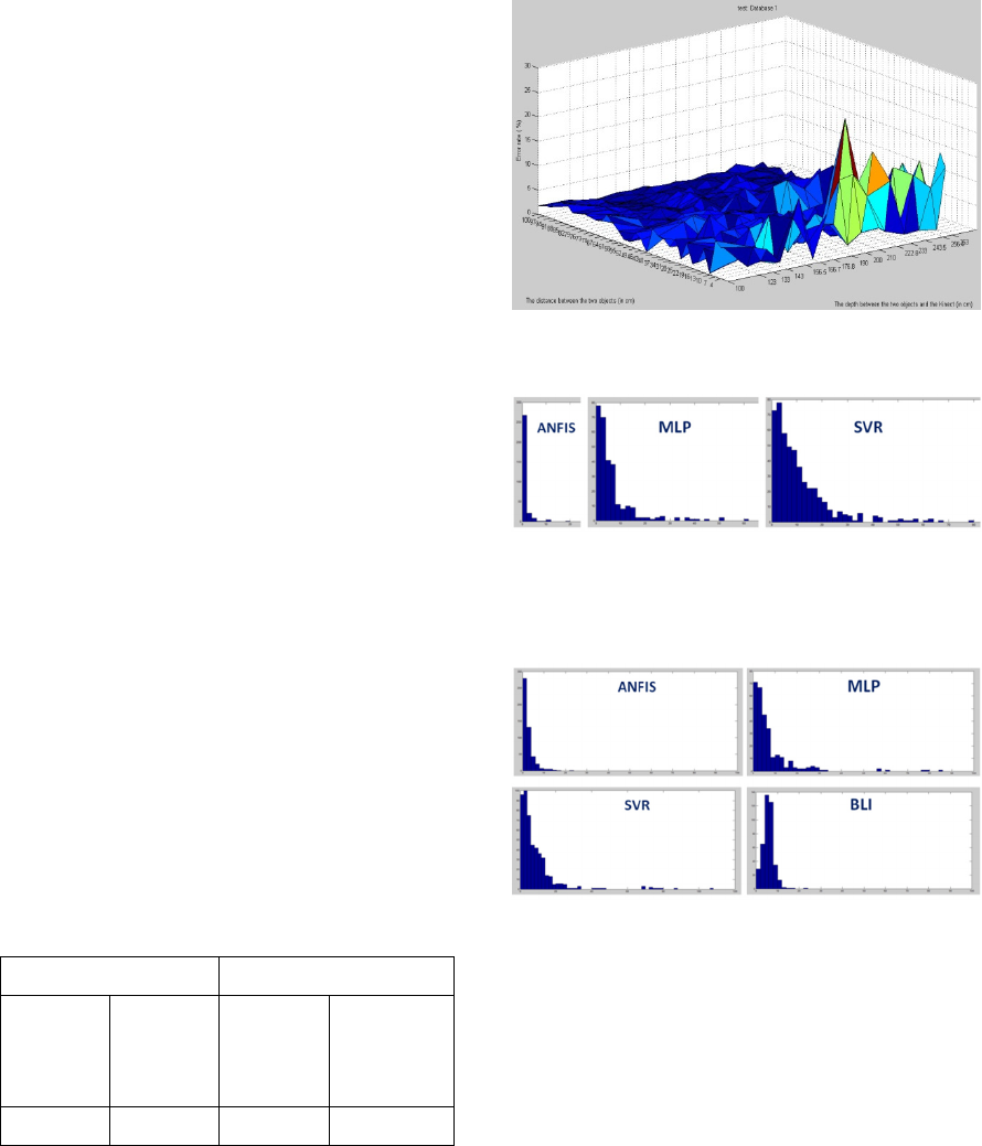
Figure 8: Example of distance estimation error in testing
Mode (ANFIS).
Figure 9: Comparison of Distance estimation error’s
distribution in Learning Mode: ANFIS (
= 1.03% /
= 1.94%), MLP (
= 6.95% /
=
10.73%) and SVR (
= 11.08% /
= 12.39%).
Figure 10: Comparison of Distance estimation error’s
distribution in Testing Mode: ANFIS (
= 2.46% /
= 2.73%), MLP (
= 7.57% /
=
11.21%), SVR (
= 8.73% /
= 12.12%) and
BLI (
= 5.70% /
= 2.58%).
5 CONCLUSIONS
The obtained distance estimation errors between two
objects in generalization mode are 2.46%, 7.57%,
8.73 and 5.70% for ANFIS, MLP, SVR and BLI,
respectively. The estimation of the distance between
two objects in centimetres using ANFIS gives better
result than the MLP, SVR and BLI. Concerning
MLP and SVR, they have been used within a
classification-like paradigm and thus lead to
generating a large number of classes. That is why
NCTA 2015 - 7th International Conference on Neural Computation Theory and Applications
172
the generalization remains quite far from expected
accuracy. Concerning the Bilinear Interpolation, this
method is based on the local approximation strategy.
In fact, the disadvantage of this method is that the
distance is calculated from the four neighbourhood
distance values and depends on the precision of
these four distances values, without the possibility of
a correction or adjustment. Although, out of
sufficient accuracy for metrological applications
(where an estimation with high precision is
required), two among the presented distance
estimation approaches, namely ANFIS-based and
BLI-based ones, present appealing features relating
robots’ navigation oriented applications.
Farther works relating the investigated technique
will concern the enhancement of the estimation
precision by using more sophisticated interpolation
techniques.
REFERENCES
Fraihat, H., Sabourin, C., Madani, K., 2015. Soft-
computing based fast visual objects’ distance
evaluation for robots’ vision. The 8
th
IEEE
International Conference on Intelligent Data
Acquisition and Advanced Computing Systems.
Hoffmann, J., Jüngel, M., & Lötzsch, M., 2005. A vision
based system for goal-directed obstacle avoidance. In
RoboCup 2004: Robot Soccer World Cup VIII (pp.
418-425). Springer Berlin Heidelberg.
Borenstein, G., 2012. Making things see: 3D vision with
kinect, processing, Arduino, and MakerBot. "O'Reilly
Media, Inc.".
Gonzalez, R. C., Woods, R. E., & Eddins, S. L., 2004.
Digital image processing using MATLAB. Pearson
Education India.
Moreno, R., Ramik, M., Graña, M., Madani, M., 2012.
"Image Segmentation on the SphericalCoordinate
Representation of the RGB Color Space", IET Image
Procession, vol. 6, no. 9, pp. 1275-1283.
Comaniciu, D., Meer, P., 2002. Mean shift: A robust
approach toward feature space analysis. Pattern
Analysis and Machine Intelligence, IEEE Transactions
on, 24(5), 603-619.
Comaniciu, D., Ramesh, V., Meer, P., 2000. Real-time
tracking of non-rigid objects using mean shift. In
Computer Vision and Pattern Recognition. IEEE
Conference on (Vol. 2, pp. 142-149).
Kheng, L. W., 2011. Mean shift tracking. Technical
report, National Univ. of Singapore.
Jyh-shing Roger Jang, Chuen-Tsai Sun, 1995. Neuro-
Fuzzy Modeling and Control.
Jang, J.-S.R., Sun, C.-T., and Mizutani, E, 1997. ‘Neuro-
fuzzy and soft computing; a computational approach
to learning and machine intelligence’.
Jyh-shing Roger Jang, 1993. ANFIS: Adaptive-Network-
based Fussy Inference System.
Rumelhart D., Hinton G., Williams R.,1986. Learning
Internal Representations by Error Propagation".
Parallel Distributed Processing: Explorations in the
Microstructure of Cognition, MIT Press.
Lippman R. P, 1987. “An Introduction to Computing with
Neural nets”, IEEE ASSP Magazine, pp. 4-22.
J. Smola et B. Scholkopf, 2004. A tutorial on support
vector regression. Statistics and Computing, pp. 199–
222.
Intel 1996. Using MMX™ Instructionsto Implement
Bilinear Interpolation of Video RGBValues.
Lu, G. Y., & Wong, D. W., 2008. An adaptive inverse-
distance weighting spatial interpolation technique.
Computers & Geosciences, 34(9), 1044-1055.
Deliang Chen, Tinghai Ou, Lebing Gong, 2010. “Spatial
interpolation of daily precipitation in China: 1951–
2005”. Advances in Atmospheric Sciences, Vol. 27,
No. 6,, pp.1221-1232.
Cok, D. R., 1987, Signal Processing Method and Appartus
for Producing Interpolated Chrominance Values in a
Sampled Color Image Signal. US Patent 4,642,678.
Vapnik, V.. The nature of statistical learning theory.
Springer, NewYork, 1995. 58, 59.
Learning-based Distance Evaluation in Robot Vision - A Comparison of ANFIS, MLP, SVR and Bilinear Interpolation Models
173
