Artificial Neural Networks for In-silico Experiments on Perception
Simon Odense
University of Victoria, Victoria, Canada
Keywords:
Computer Vision, Deep Neural Network, RTRBM.
Abstract:
Here the potential use of artificial neural networks for the purpose of understanding the biological processes
behind perception is investigated. Current work in computer vision is surveyed focusing on methods to deter-
mine how a neural network utilizes it’s resources. Analogies between feature detectors in deep neural networks
and signaling pathways in the human brain are made. With these analogies in mind, procedures are outlined
for experiments on perception using the recurrent temporal restricted Boltzmann machine as an example. The
potential use of these experiments to help explain disorders of human perception is then described.
1 INTRODUCTION
Since their inception, artificial neural networks
(ANNs) have proved to be invaluable tools for ma-
chine learning and artificial intelligence. ANNs
offer a practical implementation of computational
paradigms that resemble those found in the nervous
system. The goal of utilizing ANNs for regression
and classification tasks runs parallel to the study of
biological neural networks for the purpose of under-
standing the human brain. As ANNs and their learn-
ing algorithms grow more sophisticated, their ability
to model sensory data provides a unique opportunity
to produce insight into the workings of perception.
Here we argue that, despite being vast simplifications
of their biological counterparts, modern ANNs are
powerful enough to realistically model complicated
datasets and as such should be considered as tools
for understanding the biological process behind per-
ception. We begin by surveying existing work us-
ing ANNs in computer vision before proposing some
general experimental methods to facilitate this type of
study using the Recurrent Temporal Restricted Boltz-
mann Machine (RTRBM) as an example.
2 PARAMETER VARIATION
2.1 Reconstructions of Visual Data
using ANNs
ANNs called deep neural networks (in particular
deep convolutional neural nets) have been gaining
traction in computer vision (Krizhevsky et al., 2012).
Although capable of providing state of the art results
in image recognition, little is understood about the
representations that deep neural networks come up
with. Deep neural networks (DNNs) are made up
of a series of stacked layers of hidden units. Each
layer represents certain features of the input data with
higher layers representing more abstract features.
Lower layers map features such as edge detectors
whereas higher layers may represent specific ob-
jects. Deep neural networks form representations
of input data via hidden units. The state of the
hidden units given input data is determined by
parameters called weights and biases. Although
certain a priori knowledge of the dataset allows one
to impose useful restrictions on the parameter space,
the parameter values are selected using learning
algorithms. The result of this is that after training
a network, one doesn’t know how the weights
are used by the network to model the data. What
feature detectors a network has come up with and
which hidden units model which features is unknown.
Finding out what features a trained DNN uses
is key to understanding how they work and to
developing better networks. Recent papers have
developed methods for analyzing how DNNs use
their resources to model image data (Erhan et al.,
2009)(Mahendran and Vedaldi, 2015). One method
is based on the concept of reconstructing input data.
Suppose we have a neural network trained on a data
set X. Then given an input vector x ∈ X, we can form
a representation of x, φ(x) using the neural network.
The analysis of these representations boils down
to finding a good way of inverting φ. By design φ
will not be uniquely invertible. Nonetheless several
Odense, S..
Artificial Neural Networks for In-silico Experiments on Perception.
In Proceedings of the 7th International Joint Conference on Computational Intelligence (IJCCI 2015) - Volume 3: NCTA, pages 163-167
ISBN: 978-989-758-157-1
Copyright
c
 2015 by SCITEPRESS – Science and Technology Publications, Lda. All rights reserved
163

inversion methods have been developed for DNNs
(Mahendran and Vedaldi, 2015)(Dosovitskiy and
Brox, 2015). (Zeiler and Fergus, 2014). The nature
of these visual reconstructions can be quite striking.
This raises the question of what this procedure can
tell us about perception in the human brain.
By selectively perturbing the parameters of a trained
neural network we can sample from the reconstruc-
tions of this perturbed neural network to examine the
effects of the parameter shift. This can be seen as
a type of in-silico experiment on perception. When
the parameters can be grouped together by functional
role these perturbations can be seen as analogous
to modifying various signalling pathways in the brain.
One key problem in using DNNs for this purpose is
that DNNs have been shown to be easily “fooled”
into recognizing images that are not recognizable to
humans (Nguyen et al., 2015). With this in mind one
must be cautious in making inferences about human
vision on the basis of a single model. However, by
examining the reconstructions produced by a large
variety of different models one hopes to find certain
qualitative shifts that are present in a large number
of models. Examining the effects of parameter
shifts for a single network architecture may provide
information on how that specific architecture uses
its resources, but this may not generalize to different
kinds of ANNs. This highlights the importance
of using a wide variety of models if one wants to
identify common types of sensory distortions.
2.2 Signalling Pathways in the Human
Brain
The human brain can be seen as a large neural
network in which neurons interact via synapses. One
neuron signals another with an electrical impulse
that travels along the axon towards the synapse.
From there neurotransmitters are released which
bind to receptors on the neighbouring neuron. The
human brain contains a large number of different
neurotransmitters and their corresponding receptors
for this purpose. This gives rise to the view of the
brain as a series of interacting signalling pathways
each given by a specific neurotransmitter. Selective
alterations in the function of a specific neurotrans-
mitter can have drastic effects on both perception and
cognition. Imbalances in levels of neurotransmitters
in the brain have been implicated in a wide variety
of mental disorders from depression to schizophrenia
(Spies et al., 2015)(Howes and Kapur, 2009). Al-
though artificial neural networks are nowhere near
sophisticated enough to model the cognitive aspects
of these disorders, we argue that they are becoming
powerful enough to model the sensory aspects of
these disorders.
Varying effectiveness of neurotransmitters can
be seen as a perterbation in the signalling pathways
of the brain. We would like to recreate this type
of perturbation using ANNs. The most obvious
way to replicate this effect in an ANN is by scaling
sets of parameters by some multiplicative factor.
Although one can partition the parameters of an
ANN arbitrarily, this procedure would presumably
be more effective when parameters are grouped by
functional significance. As discussed before, in most
ANNs the weights are functionally equivalent before
training. After training, one may utilize methods
discussed in the previous section to identify distinct
functional groups of weights, for example, edge de-
tectors. ANNs are too reductionist to provide direct
analogies between their dynamics and the dynamics
of the human brain. However, experimenting with
parameter shifts in the above way may illuminate
abstract mechanisms that can produce certain types
of sensory distortion.
Some neural networks have different sets of param-
eters with pre-defined roles. That makes the process
of parameter scaling simpler as the network already
comes equipped with distinct sets of parameters. In
the following illustrative example, we use a type of
neural network with two distinct sets of parameters,
those used to communicate within a time step and
those used to communicate between time steps.
3 THE RECURRENT TEMPORAL
RESTRICTED BOLTZMANN
MACHINE
The restricted Boltzmann machine (RBM) is a type
of probabilistic artificial neural network defined over
binary vectors x = (v,h) ∈ {0, 1}
N
v
+N
h
with
P(v,h) =
exp(v
>
W h + c
>
v + b
>
h)
Z
here W is a matrix of weights, c,b are vectors of bi-
ases and N
v
,N
h
are the number of nodes for v and h
respectively, and Z is the normalizing factor. When
the visible units are real-valued the Boltzmann ma-
chine can be modified by defining
P(v,h) =
exp(v
>
W h + c
>
v + b
>
h − |v|
2
/2)
Z
NCTA 2015 - 7th International Conference on Neural Computation Theory and Applications
164

In both variations of the RBM, an algorithm called
contrastive divergence allows the gradient of the log-
likelihood of training data under the parameters of
the RBM to be calculated efficiently (Hinton, 2002).
This allows RBMs to learn an implicit distribution
over training data using gradient descent. RBMs
are often also used as the building blocks for DBNs
by stacking them in layers and training the network
greedily (Hinton et al., 2006).
The recurrent temporal restricted Boltzmann machine
(RTRBM) is a variation on the restricted Boltzmann
machine designed to model temporal sequences. The
RTRBM is defined by a probability distribution over
sequences of vectors v
T
= (v
(0)
,..., v
(t−1)
) given by
the following equations.
Q(v
T
,h
0T
) =
T −1
∏
k=1
Q(v
(k)
,h
0(k)
|h
(k−1)
)
!
Q
0
(v
(0)
,h
0
(0)
).
With
Q(v
(t)
,h
0(t)
|h
(t−1)
)
=
exp(v
(t)>
W h
0(t)
+ c
>
v
(t)
+ b
>
h
0
(t)
+ h
0(t)>
W
0
h
(t−1)
)
Z(h
(t−1)
)
,
and h
T
is a sequence of real-valued vectors defined by
h
(t)
= σ(W v
(t)
+W
0
h
(t−1)
+ b),
h
(0)
= σ(W v
(0)
+ b
init
+ b).
Here σ is the logistic function, b
init
is an initial
bias, and Z(h
(t−1)
) is a normalizing factor. The
RTRBM can be seen as a sequence of RBMs with
a dynamic hidden bias. These equations are given
by 3 distinct sets of parameters, b,W,W
0
. In the
following experiments we train an RTRBM on video
sequences of bouncing balls. The video sequences
are 30 × 30 videos generated algorithmically. Each
pixel is represented by a visible unit giving a total of
900 visible units. Training is done with 400 hidden
units for 100, 000 iterations using backpropogation
through time as done by Sutskever et al. (2008).
Given a trained RTRBM, there are two common
ways of forming representations of the input data
in the RTRBM. One can either sample from the
conditional distribution of the hidden units given
the visible units, or the hidden units can be encoded
with a mean-field approximation. Here we use the
former. We begin by sampling from the training
sequences to get an input sequence, v
T
0
. To obtain a
representation of the input sequence, we sample from
the conditional distribution over the hidden units
given the input sequence. In other words, we sample
h
0T
∼ Q(·|v
T
0
). Finally, we form the reconstructed
input sequence by using a mean field approximation
from the conditional distribution of the visible units
given the hidden sequence h
0T
. That is we set each
v
(t)
i
← Q(v
(t)
i
= 1|h
0(t)
). This procedure faithfully
reconstructs the input data v
T
0
. Next we shift the
parameters of the trained network to observe the
effects on the reconstructions. To do this we repeat
the previous process using a perterbed network, Q
α,β
,
for the first step. Q
α,β
is defined to be the distribution
produced after scaling W and W
0
by factors α and β
respectively. In other words, we sample the hidden
units from the distribution defined by
Q
α,β
(h
0(t)
i
= 1|x
(t−1)
,h
(t−1)
)
= σ(α
∑
j
w
i, j
x
(t)
j
+ β
∑
k
w
0
i,k
h
(t−1)
k
+ b
i
)
with b
init
replacing β
∑
k
w
0
i,k
h
(t−1)
k
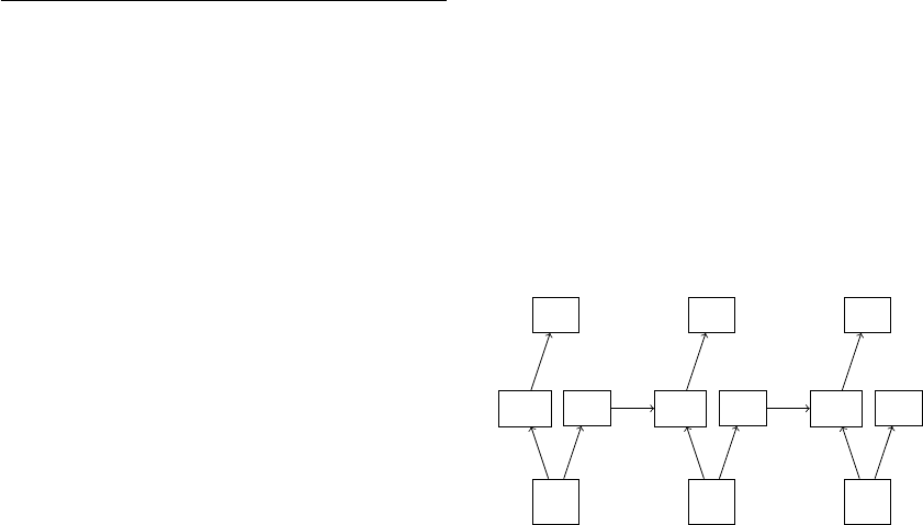
for t = 0 (see Fig.
1). Reconstructions were produced under (α, β) =
(1,1), (1,0.5), (1,0), (0.5,1),(0,1),(0.5,0.5).
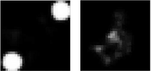
The reconstructions with scaled down temporal
weights and unchanged visible weights show the
balls very clearly but the position of the balls is erratic
and in the extreme case of (1,0) doesn’t correspond
to the position of the balls in the input sequence at
all. Interestingly, the position of the balls under (1,0)
seems to tend to the corners. When the temporal
weights are unchanged and the visible weights scaled
down the balls become indistinct and fuzzy although
the motion of the balls is smooth. In the extreme
case of (0,1) it becomes impossible to distinguish
individual balls. The reconstructions under (0.5, 0.5)
show a mixture of the two effects (see Fig. 2).
v
(0)
h
0
(0)
v
(0)
0
h
(0)
v
(1)
h
0
(1)
v
(1)
0
h
(1)
v
(2)
h
0
(2)
v
(2)
0
h
(2)
α α
β
α α
β
α α
Figure 1: The reconstruction process: Starting with a se-
quence of input vectors, v
T
0
, the hidden sequence h
0
T
is pro-
duced after scaling the parameters of the RTRBM by α and
β. From there the reconstructed sequence, v
T
, is produced
either by sampling or mean-field approximation. Note that
using a mean-field approximation to encode data in the hid-
den units amounts to using h
T
to reconstruct v
T
.
Next, the Gaussian variant of the RTRBM was
trained on the mocap data used by Taylor et al.
Artificial Neural Networks for In-silico Experiments on Perception
165

(2006). The mocap data consists of sequences of 49
position vectors The RTRBM was trained with 200
hidden units for 100,000 iterations. Reconstructions
were produced in a similar manner as before except in
the final step the reconstructed vector was produced
by setting v
(t)
← W h
0
(t)
. The reconstructions failed
to produce distinct qualitative shifts under various
parameter shifts. The reconstructions produced under
(1,0.5), (1,0) and (0.5, 1),(0.1) both show deficien-
cies in modeling the trajectory and the movement of
the raw data. This suggests that the usefulness of this
procedure depends highly on the nature of the dataset
and the ability of an observer to interpret the results.
In the RTRBM the two sets of parameters, W
and W
0
, have very clearly defined roles. Given that
we know what these roles are, the nature of the
reconstructions may be unsurprising. However, when
scaling up to natural images the results of parameter
scaling may be less obvious. This is especially
true when the feature detectors have no obvious
interpretation. This demonstrates the potential use of
ANNs to observe distinct qualitative shifts in video
data. The results of this procedure when used with
mocap data are less enlightening. This may be due
to the inability of a human observer to correctly
interpret the results. For more abstract data sets this
becomes even more problematic. However, when
dealing with datasets that correspond to sensory
information, one should be able to see whether or not
a given parameter shift induces a qualitative change
in reconstructions. Even the absence of qualitative
shifts can prove informative as it can tell you that the
set of parameters chosen doesn’t correspond to a par-
ticular feature detector and may indicate an inability
of the network to use it’s resources optimally.
Figure 2: A comparison of two sample frames from recon-
structions of the bouncing balls under scaling factors (1,0)
(on the left) and (0,1) (on the right). Under (1,0) one can
see distinct balls. However, the balls stay mostly in the cor-
ners and exhibit very erratic movement. Under (0,1) distinct
balls are no longer visible but the motion is smooth.
4 CONCLUSION
The advantage in using ANNs over more realistic
biological models is their tractability. Although
biological neural networks may serve as inspiration
for the design of ANNs, when used for practical
purposes the resmblence of an ANN to a biological
neural network is inconsequential. For this reason
many do not consider the potential of ANNs to study
the function of the human brain.
As ANNs (and DNNs in particular) become
more and more capable of modelling sensory data,
more research is being done into the mechanisms
used by DNNs to model their data. Methods have
been developed that allow one to determine what
feature detectors a DNN comes up with after training.
With a known set of feature detectors and a good
way of inverting representations, one can examine
the effect of scaling functional groups of parameters
on reconstructions of input data. The effectiveness
of this procedure is demonstrated with the simple
example of the RTRBM. In the RTRBM there are
two sets of parameters used, the temporal and visible
weights. This allows us to bypass the process of
finding feature detectors. Furthermore, a single-layer
RTRBM has a straightforward inversion process by
simply sampling the hidden units and then using a
mean-field approximation to obtain a value for the
visible units. In the RTRBM we begin with a rough
idea of how each set of parameters is going to be
used by the network to model the input data. This
makes the nature of the reconstructions somewhat
predictable. Training a network on a more com-
plicated dataset we may be interested in modifying
other sets of feature detectors that are not known to
begin with. The effect of modifying these feature
detectors on the reconstructions may be less obvious
than it is in the RTRBM.
Following the above procedure gives us a corre-
spondence between distinct qualitative shifts in visual
reconstructions with a parameter shift of certain
feature detectors. Working backwards, specific
distortions in perception may be identified by those
suffering from mental or neurological disorders. Be-
ing able to match a specific kind of shift in visual data
to a mechanism in an artificial neural network may
provide a hint as to the mechanism that malfunctions
in the human brain to produce such a distortion. As
pointed out before the identification of a shift in
visual data with a mechanism in an ANN might be
an invalid comparison, as the mechanism used by the
ANN might be specific to the particular model. This
identification is made stronger when a large number
of ANNs produce a similar shift through similar
mechanisms.
NCTA 2015 - 7th International Conference on Neural Computation Theory and Applications
166

ACKNOWLEDGEMENTS
The code used for the experiments was a mod-
ified version of the code used in the orig-
inal paper on RTRBMs by Sutskever et al.
(2008). This includes the code used to gen-
erate the video sequences of bouncing balls.
The mocap data was obtained from the sample
code provided at http://www.uoguelph.ca/ gwtay-
lor/publications/nips2006mhmublv/code.html
REFERENCES
Dosovitskiy, A. and Brox, T. (2015). Inverting convolu-
tional networks with convolutional networks. Techni-
cal report. arXiv:1506.02753.
Erhan, D., Bengio, Y., Courville, A., and Vincent, P. (2009).
Visualizing higher-layer features of a deep network.
Technical Report 1341, University of Montreal.
Hinton, G. (2002). Training a product of experts by mini-
mizing contrastive divergence. Neural Computation,
14(8):1771–1800.
Hinton, G., Osindero, S., and Teh, Y. (2006). A fast learning
algorithm for deep belief networks. Neural Computa-
tion, 18:1527–1553.
Howes, O. and Kapur, S. (2009). The dopamine hypothesis
of schizophrenia: Version iii–the final common path-
way. Schizophrenia Bulletin, 35(3).
Krizhevsky, A., Sutskever, I., and Hinton, G. (2012). Im-
agenet classification with deep convolutional neural
networks. volume 25.
Mahendran, A. and Vedaldi, A. (2015). Understanding deep
image representations by inverting them. Computer
Vision and Pattern Recognition.
Nguyen, A., Yosinski, J., and Clune, J. (2015). Deep neu-
ral networks are easily fooled: High confidence pre-
dictions for unrecognizable images. Computer vision
and Pattern Recognition, arXiv:1412.1897v4.
Spies, M., Knudsen, G., Lanzenberger, R., and Kasper, S.
(2015). The serotonin transporter in psychiatric disor-
ders: Insights from pet imaging. The Lancet Psychia-
try, 2(8):743–55.
Sutskever, I., Hinton, G., and Taylor, G. (2008). The re-
current temporal restricted boltzmann machine. vol-
ume 21.
Taylor, G., Hinton, G., and Roweis, S. (2006). Modeling hu-
man motion using binary latent variables. volume 19.
Zeiler, M. and Fergus, R. (2014). Visualizing
and understand convolutional networks. ECCV,
arXiv:1311.2901.
Artificial Neural Networks for In-silico Experiments on Perception
167