Piecewise Chebyshev Factorization based Nearest Neighbour
Classification for Time Series
Qinglin Cai, Ling Chen and Jianling Sun
College of Computer Science and Technology, Zhejiang University, Hangzhou, China
Keywords: Time Series, Piecewise Approximation, Similarity Measure.
Abstract: In the research field of time series analysis and mining, the nearest neighbour classifier (1NN) based on
dynamic time warping distance (DTW) is well known for its high accuracy. However, the high
computational complexity of DTW can lead to the expensive time consumption of classification. An
effective solution is to compute DTW in the piecewise approximation space (PA-DTW), which transforms
the raw data into the feature space based on segmentation, and extracts the discriminatory features for
similarity measure. However, most of existing piecewise approximation methods need to fix the segment
length, and focus on the simple statistical features, which would influence the precision of PA-DTW. To
address this problem, we propose a novel piecewise factorization model for time series, which uses an
adaptive segmentation method and factorizes the subsequences with the Chebyshev polynomials. The
Chebyshev coefficients are extracted as features for PA-DTW measure (ChebyDTW), which are able to
capture the fluctuation information of time series. The comprehensive experimental results show that
ChebyDTW can support the accurate and fast 1NN classification.
1 INTRODUCTION
In the research field of time series analysis and
mining, time series classification is an important
task. A plethora of classifiers have been developed
for this task (Esling et al, 2012; Fu, 2011), e.g.,
decision tree, nearest neighbor (1NN), naive Bayes,
Bayesian network, random forest, support vector
machine, etc. However, the recent empirical
evidence (Ding et al, 2008; Hills et al, 2014; Serra et
al, 2014) strongly suggests that, with the merits of
robustness, high accuracy, and free parameter, the
simple 1NN classifier employing generic time series
similarity measure is exceptionally difficult to beat.
Besides, due to the high precision of dynamic time
warping distance (DTW), the 1NN classifier based
on DTW has been found to outperform an
exhaustive list of alternatives (Serra et al, 2014),
including the decision trees, the multi-scale
histograms, the multi-layer perception neural
networks, the order logic rules with boosting, as well
as the 1NN classifiers based on many other
similarity measures. However, the computational
complexity of DTW is quadratic to the time series
length, i.e., O(n
2
), and the 1NN classifier has to
search the entire dataset to classify an object. As a
result, the 1NN classifier based on DTW is low
efficient for the high-dimensional time series. To
address this problem, researchers have proposed to
compute DTW in the alternative piecewise
approximation space (PA-DTW) (Keogh et al, 2001;
Keogh et al, 2004; Chakrabarti et al, 2002; Gullo et
al, 2009), which transforms the raw data into the
feature space based on segmentation, and extracts
the discriminatory and low-dimensional features for
similarity measure. If the original time series with
length n is segmented into N (N << n) subsequences,
the computational complexity of PA-DTW will
reduce to O(N
2
).
Many piecewise approximation methods have
been proposed so far, e.g., piecewise aggregation
approximation (PAA) (Keogh et al, 2001), piecewise
linear approximation (PLA) (Keogh et al, 2004;
Keogh et al, 1999), adaptive piecewise constant
approximation (APCA) (Chakrabarti et al, 2002),
derivative time series segment approximation (DSA)
(Gullo et al, 2009), piecewise cloud approximation
(PWCA) (Li et al, 2011), etc. The most prominent
merit of piecewise approximation is the ability of
capturing the local characteristics of time series.
However, most of the existing piecewise
approximation methods need to fix the segment
84
Cai, Q., Chen, L. and Sun, J..
Piecewise Chebyshev Factorization based Nearest Neighbour Classification for Time Series.
In Proceedings of the 7th International Joint Conference on Knowledge Discovery, Knowledge Engineering and Knowledge Management (IC3K 2015) - Volume 1: KDIR, pages 84-91
ISBN: 978-989-758-158-8
Copyright
c
 2015 by SCITEPRESS – Science and Technology Publications, Lda. All rights reserved

length, which is hard to be predefined for the
different kinds of time series, and focus on the
simple statistical features, which only capture the
aggregation characteristics of time series. For
example, PAA and APCA extract the mean values,
PLA extracts the linear fitting slopes, and DSA
extracts the mean values of the derivative
subsequences. If PA-DTW is computed on these
methods, its precision would be influenced.
In this paper, we propose a novel piecewise
factorization model for time series, named piecewise
Chebyshev approximation (PCHA), where a novel
code-based segmentation method is proposed to
adaptively segment time series. Rather than focusing
on the statistical features, we factorize the
subsequences with Chebyshev polynomials, and
employ the Chebyshev coefficients as features to
approximate the raw data. Besides, the PA-DTW
based on PCHA (ChebyDTW) is proposed for the
1NN classification. Since the Chebyshev
polynomials with different degrees represent the
fluctuation components of time series, the local
fluctuation information can be captured from time
series for the ChebyDTW measure. The
comprehensive experimental results show that
ChebyDTW can support the accurate and fast 1NN
classification.
2 RELATED WORK
2.1 Data Representation
In many application fields, the high dimensionality
of time series has limited the performance of a
myriad of algorithms. With this problem, a great
number of data approximation methods have been
proposed to reduce the dimensionality of time series
(Esling et al, 2012; Fu, 2011). In these methods, the
piecewise approximation methods are prevalent for
their simplicity and effectiveness. The first attempt
is the PAA representation (Keogh et al, 2001),
which segments time series into the equal-length
subsequences, and extracts the mean values of the
subsequences as features to approximate the raw
data. However, the extracted single sort of features
only indicates the height of the subsequences, which
may cause the local information loss. Consecutively,
an adaptive version of PAA, named piecewise
constant approximation (APCA) (Chakrabarti et al,
2002), was proposed, which can segment time series
into the subsequences with adaptive lengths and thus
can approximate time series with less error. As well,
a multi-resolution version of PAA, named MPAA
(Lin et al, 2005), was proposed, which can
iteratively segment time series into 2
i
subsequences.
However, both of the variations inherit the poor
expressivity of PAA. Another pioneer piecewise
representation is the PLA (Keogh et al, 2004; Keogh
et al, 1999), which extracts the linear fitting slopes
of the subsequences as features to approximate the
raw data. However, the fitting slopes only reflect the
movement trends of the subsequences. For the time
series fluctuating sharply with high frequency, the
effect of PLA on dimension reduction is not
prominent. In addition, two novel piecewise
approximation methods were proposed recently. One
is the DSA representation (Gullo et al, 2009), which
takes the mean values of the derivative subsequences
of time series as features. However, it is sensitive to
the small fluctuation caused by the noise. The other
is the PWCA representation (Li et al, 2011), which
employs the cloud models to fit the data distribution
of the subsequences. However, the extracted features
only reflect the data distribution characteristics and
cannot capture the fluctuation information of time
series.
2.2 Similarity Measure
DTW (Esling et al, 2012; Fu, 2011; Serra et al,
2014) is one of the most prevalent similarity
measures for time series, which is computed by
realigning the indices of time series. It is robust to
the time warping and phase-shift, and has high
measure precision. However, it is computed by the
dynamic programming algorithm, and thus has the
expensive O(n
2
) computational complexity, which
largely limits its application to the high dimensional
time series (Rakthanmanon et al, 2012). To
overcome this shortcoming, the PA-DTW measures
were proposed. The PAA representation based
PDTW (Keogh et al, 2000) and the PLA
representation based SDTW (Keogh et al, 1999) are
the early pioneers, and the DSA representation based
DSADTW (Gullo et al, 2009) is the state-of-the-art
method. Rather than in the raw data space, they
compute DTW in the PAA, PLA, and DSA spaces
respectively. Since the segment numbers are much
less than the original time series length, the PA-
DTW methods can greatly decrease the
computational complexity of the original DTW.
Nonetheless, the precision of PA-DTWs greatly
depends on the used piecewise approximation
methods, where both the segmentation method and
the extracted features are crucial factors. As a result,
with the weakness of the existing piecewise
approximation methods, the PA-DTWs cannot
Piecewise Chebyshev Factorization based Nearest Neighbour Classification for Time Series
85

achieve the high precision. In our proposed
ChebyDTW, a novel adaptive segmentation method
and the Chebyshev factorization are used, which
overcomes the drawback of the fixed segmentation,
and can capture the fluctuation information of time
series for similarity measure.
3 PIECEWISE FACTORIZATION
Without loss of generality, we first give the relevant
definitions as follows.
Definition 1. (Time Series): The sample
sequence of a variable X over n contiguous time
moments is called time series, denoted as T = {t
1
, t
2
,
…, t
i
, …, t
n
}, where t
i
∈
R denotes the sample value
of X on the i-th moment, and n is the length of T.
Definition 2. (Subsequence): Given a time series
T = {t
1
, t
2
, …, t
i
, …, t
n
}, the subset S of T that
consists of the continuous samples {t
i+1
, t
i+2
, …, t
i+l
},
where 0 ≤ i ≤ n-l and 0 ≤ l ≤ n, is called the
subsequence of T.
Definition 3. (Piecewise Approximation
Representation): Given a time series T = {t
1
, t
2
, …,
t
i
, …, t
n
}, which is segmented into the subsequence
set S = {S
1
, S
2
, …, S
j
, …, S
N
}, if ∃ f: S
j
→ V
j
= [v
1
, ...,
v
m
]
∈
R
m
, then the set V = {V
1
, V
2
, …, V
j
, …, V
N
} is
called the piecewise approximation of T.
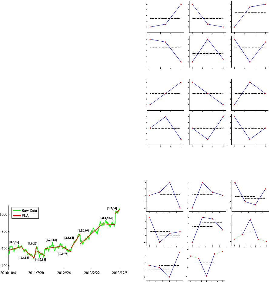
Figure 1 shows the example of PLA
representation (in red), for the stock price time series
(in green) of Google Inc. (symbol: GOOG) from The
NASDAQ Stock Market, which consists of the close
prices at 800 consecutive trading days
(2010/10/4~2013/12/5). As shown, PLA takes the
linear fitting slopes and the spans of the
subsequences as features to approximate the raw
data, e.g., [0.5, 96] for the first subsequence.
Figure 1: The PLA representation for the stock price time
series.
3.1 Adaptive Segmentation
Inspired by the Marr's theory of vision (Ullman et al,
1982), we regard the turning points, where the trend
of time series changes, as a good choice to segment
time series. However, the practical time series is
mixed with a mass of noise, which results in many
trivial turning points with small fluctuation. This
problem can be simply solved by the efficient
moving average (MA) smoothing method (Gao et al,
2010).
(a)
(b)
Figure 2: Three adjacent samples with the cell codes of (a)
basic relationships, and (b) specific relationships.
Figure 3: The minimum turning patterns composed with
two cell codes.
In order to recognize the significant turning
points, we first exhaustively enumerate the location
001-110 011-100
100-001
100-011
011-110
110-001
0
0
μ
0
0
0
1
1
011
110
1
0
010
1
0
0
1
100
1
001
001
0
110
0
1
1
0
0
1
010
0
1
1
0
1
010
0
μ
1
0
1 1
101
1
0
101
1
0
1
101
101
010
KDIR 2015 - 7th International Conference on Knowledge Discovery and Information Retrieval
86

relationships of three adjacent samples t
1
-t
3
with
their mean μ in time series, as shown in Figure 2. Six
basic cell codes can be defined as Figure 2(a), which
is composed by the binary codes δ
1
-δ
3
of t
1
-t
3
, and
denoted as Φ(t
1
, t
2
, t
3
) = (δ
1
δ
2
δ
3
)
b
. Six special
relationships that one of t
1
-t
3
equals to μ are encoded
as Figure 2(b).
Based on the cell codes, all the minimum turning
patterns (composed with two cell codes) at the
turning points can be enumerated as Figure 3. Note
that, the basic cell codes 010 and 101 per se are the
turning patterns. Then, we employ a sliding window
with length 3 to scan the time series, and encode the
samples within each window by Figure 2. In this
process, all the significant turning points can be
found by matching Figure 3, with which time series
can be segmented into the subsequences with the
adaptive lengths.
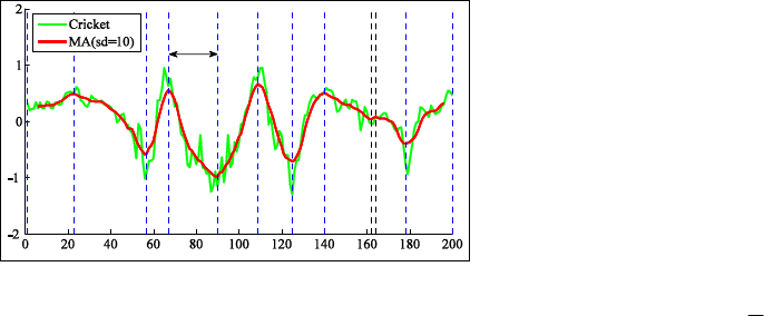
However, the above segmentation is not perfect.
Although the trivial turning points can be removed
with the MA, the "singular" turning patterns may
exist, i.e., the turning patterns appearing very close.
As shown in Figure 4, a Cricket time series from the
UCR time series archive (Keogh et al, 2011) is
segmented by the turning patterns (dash line), where
the raw data is first smoothed with the smooth
degree 10 (sd = 10).
Figure 4: Segmentation for the Cricket time series.
Obviously, the dash lines can significantly
segment the time series, but the two black dash lines
are so close that the segment between them can be
ignored. In view of this, we introduce the segment
threshold ρ that stipulates the minimum segment
length. This parameter can be set as the ratio to the
time series length. Since the time series from a
specific filed exhibit the same fluctuation
characteristics, ρ is data-adaptive and can be learned
from the labeled dataset. Nevertheless, the
segmentation is still primarily established on the
recognition of turning patterns, which determines the
segment number or lengths adaptively, and is
essentially different from the principles of the
existing segmentation methods.
3.2 Chebyshev Factorization
At the beginning, it is necessary to z-normalize the
obtained subsequences as a pre-processing step.
Rather than focusing on the statistical features,
PCHA will factorize each subsequence with the first
kind of Chebyshev polynomials, and take the
Chebyshev coefficients as features. Since the
Chebyshev polynomials with different degrees
represent the fluctuation components, the local
fluctuation information of time series can be
captured in PCHA.
The first kind of Chebyshev polynomials are
derived from the trigonometric identity T
n
(cos(θ)) =
cos(nθ), which can be rewritten as a polynomial of
variable t with degree n, as Formula (1).





−≤−−
≥
−∈
=
−
−
−
1 )),(coshcosh()1(
1 )),(coshcosh(
]1 ,1[ )),(coscos(
)(
1
1
1
ttn
ttn
ttn
tT
n
n
(1)
For the sake of consistent approximation, we
only employ the first sub-expression to factorize the
subsequences, which is defined over the interval [-1,
1]. With the Chebyshev polynomials, a function F(t)
can be factorized as Formula (2).

=
≅
n
i
ii
tTctF
0
)()(
(2)
The approximation is exact if F(t) is a
polynomial with the degree of less than or equal to
n. The coefficients c
i
can be calculated from the
Gauss-Chebyshev Formula (3), where k is 1 for c
0
and 2 for the other c
i
, and t
j
is one of the n roots of
T
n
(t), which can be get from the formula t
j
= cos[(j-
0.5)π/n].

=
=
n
j
jiji
tTtF
n
k
c
1
)()(
(3)
However, the employed Chebyshev polynomials
are defined over the interval [-1, 1]. If the
subsequences are factorized with this "interval
function", they must be scaled into the time interval
[-1, 1]. Besides, the Chebyshev polynomials are
defined everywhere in the interval, but time series is
a discrete function, whose values are defined only at
the sample moments. To compute the Chebyshev
coefficients, we would process each subsequence
with the method proposed in (Cai et al, 2004), which
can extend time series into an interval function.
Given a scaled subsequence S = {(v
1
, t
1
), ..., (v
m
, t
m
)},
ρ
Piecewise Chebyshev Factorization based Nearest Neighbour Classification for Time Series
87

where -1 ≤ t
1
< ... < t
m
≤ 1, we first divide the
interval [-1, 1] into m disjoint subintervals as follows:









=
+
−≤≤
+
=
+
−
=
−
+−
mi
tt
mi
tttt
i
tt
I
mm
iiii
i
],1,
2
[
12),
2
,
2
,
[
1),
2
,1[
1
11
21
Then, the original subsequence can be extended
into a step function as Formula (4), where each
subinterval [t
i
, t
i+1
] is divided by the mid-point
(t
i
+t
i+1
)/2. The first half takes the value v
i
, and the
second half takes v
i+1
.
miItvtF
ii
≤≤∈= 1 , ,)(
(4)
After the above processing, the Chebyshev
coefficients c
i
can be computed. For the sake of
dimension reduction, we only take the first several
coefficients to approximate the raw data, which can
reflect the principal fluctuation components of time
series.
In the entire procedure, the time series needs to
be scanned only once for the adaptive segmentation
and factorization. Thus, the computational
complexity of piecewise factorization is O(kn),
where k is the extracted Chebyshev coefficient
number and much less than the time series length n.
4 SIMILARITY MEASURE
DTW is one of the most prevalent similarity
measures for time series (Serra et al, 2014), which
can find the optimal alignment between time series
by the dynamic programming algorithm. Given a
sample space F, time series T = {t
1
, t
2
, …, t
i
, …, t
m
}
and Q = {q
1
, q
2
, …, q
j
, …, q
n
}, t
i
, q
j
∈ F, a local
distance measure d: (x, y) →
R
+
should be first set in
DTW for measuring two samples. Then, a distance
matrix
C ∈ R
m×n
is computed, where each cell
records the distance between each pair of samples
from T and Q respectively, i.e.,
C(i, j) = d(t
i
, q
j
).
There is an optimal warping path in
C, which has the
minimal sum of the cells.
Definition 4. (Warping Path): Given the distance
matrix
C ∈ R
m×n
, if the sequence p = {c
1
, ..., c
l
, ...,
c
L
}, where c
l
= (a
l
, b
l
)
∈
[1 : n] × [1 : m] for l
∈
[1 :
L], satisfies the conditions that:
i) c
1
= (1, 1) and c
L
= (m, n);
ii) c
l+1
− c
l
∈
{(1, 0), (0, 1), (1, 1)} for l
∈
[1 :
L−1];
iii) a
1
≤ a
2
≤ ... ≤ a
L
and b
1
≤ b
2
≤ ... ≤ b
L
;
Then, p is called warping path. The sum of cells
in p is defined as Formula (5).
)()()(
21 Lp
cccΦ CCC +++= 
(5)
Definition 5. (Dynamic Time Warping Distance):
Given the distance matrix
C ∈ R
m×n
over time series
T and Q, and its warping path set
P = {p
1
, …, p
i
, …,
p
x
}, i, x ∈ R
+
, the minimal sum of the cells in the
warping paths Φ
min
= {Φ
ξ
|Φ
ξ
≤ Φ
λ
, ξ, λ ∈ P} is
defined as the DTW distance between T and Q.
Based on PCHA, we propose a novel PA-DTW
measure, named ChebyDTW. The algorithm of
ChebyDTW contains two layers: subsequence
matching and dynamic programming computation.
Figure 5(a) shows the dynamic programming table
with the optimal-aligned path (red shadow) of
ChebyDTW, against that of the original DTW in
Figure 5(b). In Figure 5(a), each cell of the table
records the subsequence matching result over the
Chebyshev coefficients. By the intuitive comparison,
ChebyDTW would have much lower computational
complexity than the original DTW.
With high computational efficiency, the squared
Euclidean distance is a proper measure for the
subsequence matching. Given d Chebyshev
coefficients are employed in PCHA, for
subsequences S
1
and S
2
, respectively approximated
as
C = [c
1
, ..., c
d
] and Ĉ =[ĉ
1
, ..., ĉ
d
], the squared
Euclidean distance between them can be computed
as Formula (6).

=
−=
d
i
ii
ccD
1
2
)
ˆ
()
ˆ
,( CC
(6)
Over the subsequence matching, the dynamic
programming computation performs. Given that
time series T with length m is segmented into M
subsequences, and time series Q with length n is
segmented into N subsequences, ChebyDTW can be
computed as Formula (7). C
T
and C
Q
are the PCHA
representations of T and Q respectively; C
1
T
and C
1
Q
are the first coefficient vectors of C
T
and C
Q
respectively; rest(C
T
) means the rest coefficient
vectors of C
T
except for C
1
T
; the same meaning is
taken for rest(C
Q
).





















+
==∞
==
=
otherwise
restrestChebyDTW
restChebyDTW
restChebyDTW
CCD
nm
nm
Q
T
ChebyDT
W
QT
QT
QT
QT
,
)](),([
)],(,[
],),([
min),(
0or 0 if ,
0 if ,0
),(
11
CC
CC
CC
(7)
KDIR 2015 - 7th International Conference on Knowledge Discovery and Information Retrieval
88

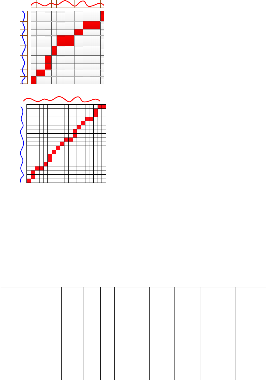
(a)
(b)
Figure 5: (a) The dynamic programming table with the
optimal-aligned path (red shadow) of ChebyDTW, (b)
against that of the original DTW.
5 EXPERIMENTS
We evaluate the 1NN classifier based on
ChebyDTW from the aspects of accuracy and
efficiency respectively. 12 real-world datasets
provided by the UCR time series archive (Keogh et
al, 2011) are employed, as shown in Table 1, which
come from various application domains and are
characterized by different series profiles and
dimensionality. All datasets have been z-normalized
and partitioned into training and testing sets by the
provider. Besides, we take the 1NN classifiers
respectively based on four prevalent PA-DTWs as
baselines, i.e., PDTW, SDTW, APCADTW, and
DSADTW. All parameters in the measures are
learned on the training datasets by the DIRECT
global optimization algorithm (Björkman et al,
1999), which is used to seek for the global minimum
of multivariate function within a constraint domain.
The experiment environment is Intel(R) Core(TM)
i5-2400 CPU @ 3.10GHz; 8G Memory; Windows 7
64-bit OS; MATLAB 8.0_R2012b.
5.1 Accuracy
Table 1 shows the 1NN classification accuracy (acc.)
based on the above PA-DTWs. The best result on
each dataset is highlighted in bold. The learned
parameters are also presented, which could make
each classifier achieve the highest accuracy on each
training dataset, including the segment threshold (ρ),
the smooth degree (sd), and the extracted Chebyshev
coefficient number (θ). For the sake of
dimensionality reduction, we learn the parameter θ
in the range of [1, 10] for ChebyDTW.
It is clear that, the 1NN classifier based on
ChebyDTW wins all datasets and has the highest
accuracy. Its superiority mainly derives from the
distinctive features extracted in ChebyDTW, which
can capture the fluctuation information for similarity
measure. Whereas the statistical features extracted in
the baselines only focus on the aggregation
characteristics of time series, which would result in
much fluctuation information loss.
Table 1: 1NN classification accuracy results based on five PA-DTWs.
Dataset
ρ sd θ
ChebyDTW PDTW SDTW APCADTW DSADTW
Adiac 0.21 22 9
0.72
0.61 0.34 0.28 0.38
Beef 0.18 17 5
0.57
0.50 0.57 0.57 0.47
CBF 0.98 8 10
0.98 0.98
0.95 0.91 0.50
ChlorineConcentration 0.73 25 8
0.65
0.60 0.55 0.56 0.62
CinC_ECG_torso 0.29 4 9
0.81
0.65 0.63 0.61 0.63
Coffee 0.51 14 9
0.89
0.79 0.75 0.82 0.61
ECG200 0.80 7 9
0.89
0.80 0.83 0.77 0.81
ECGFiveDays 0.73 17 9
0.91
0.79 0.68 0.68 0.57
FaceAll 0.51 29 10
0.73
0.63 0.50 0.63 0.71
FacesUCR 0.51 4 6
0.80
0.60 0.57 0.72 0.70
ItalyPowerDemand 0.51 7 5
0.94
0.93 0.80 0.90 0.87
SonyAIBORobotSurface 0.95 25 6
0.80
0.76 0.73 0.76 0.70
Piecewise Chebyshev Factorization based Nearest Neighbour Classification for Time Series
89

Table 2: The DCR results of five PA-DTWs.
Dataset
n
ChebyDTW PDTW SDTW APCADTW DSADTW
w DCR w DCR w DCR w DCR w DCR
Adiac 176 3.99
44.13
36 4.89 13 13.54 43 4.10 70.00 2.51
Beef 470 5.18
90.68
61 7.70 10 47.00 61 7.70 192.32 2.44
CBF 128 1.00
128.0
30 4.27 27 4.74 15 8.53 46.19 2.77
ChlorineConcentration 166 2.00
83.00
36 4.61 29 5.72 34 4.88 64.77 2.56
CinC_ECG_torso 1639 4.00
409.9
103 15.91 94 17.44 84 19.51 655.49 2.50
Coffee 286 2.00
143.0
60 4.77 33 8.67 40 7.15 117.34 2.44
ECG200 96 1.93
49.74
14 6.86 19 5.05 23 4.17 35.84 2.68
ECGFiveDays 136 1.61
84.43
9 15.11 9 15.11 5 27.20 48.24 2.82
FaceAll 131 2.00
65.50
32 4.09 32 4.09 32 4.09 53.96 2.43
FacesUCR 131 2.00
65.50
24 5.46 32 4.09 31 4.23 54.43 2.41
ItalyPowerDemand 24 1.98
12.13
5 4.80 6 4.00 6 4.00 10.61 2.26
SonyAIBORobotSurface 70 1.00
70.00
13 5.38 9 7.78 8 8.75 27.41 2.55
5.2 Efficiency
Since the efficiency of 1NN classifier is determined
by the used similarity measure, we perform the
efficiency evaluation by comparing the
computational efficiency of ChebyDTW against the
baseline PA-DTWs. The speedup of computational
complexity gained by PA-DTW over the original
DTW is O(n
2
/w
2
), where n is the time series length,
and w is the segment number. It is positively
correlated with the data compression rate (DCR =
n/w) of piecewise approximation over the raw data.
In Table 2, we present the DCRs of five PA-DTWs
on all datasets, as well as n and w. Since
ChebyDTW and DSADTW both employ the
adaptive segmentation method, the average segment
numbers on each dataset are computed for them.
As shown by the results, the DCRs of
ChebyDTW are not only much larger than the
baselines on all datasets, but also robust to the time
series length. Thus, it has the highest computational
efficiency among the five PA-DTWs. The efficiency
superiority of ChebyDTW mainly derives from the
precise approximation of PCHA over the raw data,
and the data-adaptive segmentation method, which
can segment time series into the less number of
subsequences with the adaptive lengths.
6 CONCLUSIONS
We proposed a novel piecewise factorization model
for time series, i.e., PCHA, where a novel adaptive
segmentation method was proposed, and the
subsequences were factorized with the Chebyshev
polynomials. We employed the Chebyshev
coefficients as features for PA-DTW measure, and
thus proposed the ChebyDTW for 1NN
classification. The comprehensive experimental
results show that ChebyDTW can support the
accurate and fast 1NN classification.
ACKNOWLEDGEMENTS
This work was funded by the Ministry of Industry
and Information Technology of China (No.
2010ZX01042-002-003-001), China Knowledge
Centre for Engineering Sciences and Technology
(No. CKCEST-2014-1-5), and National Natural
Science Foundation of China (No. 61332017).
REFERENCES
Esling P., Agon C., 2012. Time-series data mining. ACM
Computer Survey, 45(1).
Fu T., 2011. A review on time series data mining.
Engineering Applacations of Artificial Intelligence,
24(1): 164-181.
Ding H., Trajcevski G., Scheuermann P., Wang X., Keogh
E., 2008. Querying and mining of time series data:
experimental comparison of representations and
distance measures. In Proceedings of the VLDB
Endowment, New Zealand, pp. 1542-1552.
Hills J., Lines J., Baranauskas E., Mapp J., Bagnall A.,
2014. Classification of time series by shapelet
transformation. Data Mining and Knowledge
Discovery, 28(4): 851-881.
Serra J., Arcos J L., 2014. An empirical evaluation of
similarity measures for time series classification.
Knowledge-Based System, 67: 305-314.
Keogh E., Chakrabarti K., Pazzani M., Mehrotra S., 2001.
Dimensionality reduction for fast similarity search in
large time series databases. Knowledge Information
System, 3(3): 263-286.
KDIR 2015 - 7th International Conference on Knowledge Discovery and Information Retrieval
90

Keogh E., Chu S., Hart D., Pazzani M., 2004. Segmenting
time series: A survey and novel approach. Data
Mining in Time Series Databases. London: World
Scientific.
Chakrabarti K., Keogh E., Mehrotra S., Pazzani M., 2002.
Locally adaptive dimensionality reduction for
indexing large time series databases. ACM
Transactions on Database System, 27(2): 188-228.
Gullo F., Ponti G., Tagarelli A., Greco S., 2009. A time
series representation model for accurate and fast
similarity detection. Pattern Recognition, 42(11):
2998-3014.
Li H., Guo C., 2011. Piecewise cloud approximation for
time series mining. Knowledge-Based System, 24(4):
492-500.
Ullman S., Poggio T., 1982. Vision: A computational
investagation into the human representation and
processing of visual information, MIT Press.
Gao J., Sultan H., Hu J., Tung W., 2010. Denoising
nonlinear time series by adaptive filtering and wavelet
shrinkage: a comparison. IEEE Signal Processing
Letters, 17(3): 237-240.
Keogh E., Zhu Q., Hu B., Hao. Y., Xi X., Wei L.,
Ratanamahatana C. A., 2011. UCR time series
classification/clustering homepage:
www.cs.ucr.edu/~eamonn/time_series_data/.
Cai Y., Ng R., 2004. Indexing spatio-temporal trajectories
with Chebyshev polynomials. In Proceedings of the
2004 ACM SIGMOD international conference on
Management of data, France, pp. 599-610.
Björkman M., Holmström K., 1999. Global optimization
using the DIRECT algorithm in matlab. Advanced
Model. Optimization, 1(2): 17-37.
Keogh E., Pazzani M. J., 1999. Relevance feedback
retrieval of time series data. In Proceedings of the
22nd annual international ACM SIGIR conference on
Research and development in information retrieval,
USA, pp. 183-190.
Lin J., Vlachos M., Keogh E., 2005. A MPAA-based
iterative clustering algorithm augmented by nearest
neighbors search for time-series data streams.
Advances in Knowledge Discovery and Data Mining.
Springer Berlin Heidelberg.
Rakthanmanon T., Campana B., Mueen A., 2012.
Searching and mining trillions of time series
subsequences under dynamic time warping. In
Proceedings of the 18th ACM SIGKDD International
Conference on Knowledge Discovery and Data
Mining, China, pp. 262-270.
Keogh E. J., Pazzani M. J., 2000. Scaling up dynamic time
warping for data mining applications. In Proceedings
of the 6th ACM SIGKDD International Conference on
Knowledge Discovery and Data Mining, USA, pp.
285-289.
Keogh E. J., Pazzani M. J., 1999. Scaling up dynamic time
warping to massive datasets. Principles of Data
Mining and Knowledge Discovery. Springer Berlin
Heidelberg.
Piecewise Chebyshev Factorization based Nearest Neighbour Classification for Time Series
91