A Generic Interface Specification for Standardized Retrieval and

Statistical Evaluation of Spatial and Temporal Data

Jens Kohlmorgen

Fraunhofer Institute for Open Communication Systems FOKUS, Kaiserin-Augusta-Allee 31, 10589, Berlin, Germany

Keywords: Generic, Interface, Specification, Retrieval, Aggregation, Statistical Evaluation, Spatial, Temporal,

Spatio-Temporal, Measurement, Data.

Abstract: The interface defined in this paper provides a generic way to select, structure, aggregate, and retrieve

spatially and/or temporally localized measurement data from an underlying database in a standardized

manner. It is generic in the sense that it is neither specific to a particular type of database, nor is it specific

to a particular programming language or data format. The interface is particularly designed for software

systems where statistical analyses of potentially large collections of scalar measurement data are to be

performed by loosely coupled client applications. A key feature of the interface design is that a statistical

aggregation and evaluation of the data is performed on the server side, such that the necessary amount of

data to be transferred to a querying client is minimized. This can be a crucial feature for clients that are

querying large databases remotely, for example, over the Internet. The interface delivers regularly arranged

data to facilitate statistical assessments (e.g., visualizations in charts). It does not require, however, that the

raw data is arranged regularly in any way. In particular, measurements are not required to be synchronous or

equally spaced. The proposed interface can be employed for a wide range of application areas, e.g., to

evaluate data from sensor networks measuring the street traffic, the water and energy supply, the air

pollution or climate indicators.

1 INTRODUCTION

The widespread use of (geo-)spatially and tempo-

rally localized data in software applications has long

since driven standardization efforts towards open

standards for managing and exchanging such data.

In particular the work of the Open Geospatial

Consortium (OGC) (www.opengeospatial.org) and

the ISO technical committee ISO/TC 211

(www.isotc211.org) led to a series of international

standards and technical specifications that were

gradually incorporated into the ISO 19100 series of

standards (www.isotc211.org/Outreach/Overview/

Overview.htm). Today there exists a large number of

these comprehensive standards for many aspects of

handling geospatial data. Software services that

provide general access to such kind of data, in

particular Web services (Alonso, G., et al., 2004)

that are publicly accessible over the Internet, clearly

benefit from adopting these broadly accepted

standards. On the other hand, for services that

provide data only internally within a self-contained

software system based on a service-oriented

architecture (SOA) (Erl, T., 2005), the adoption of

these elaborate standards may prove to be

unnecessarily complex.

In particular for the latter purpose we here

propose a significantly less complex interface. It is

designed for the structured retrieval and statistical

evaluation of spatial and temporal measurements of

scalar quantities provided by a software service.

Such data is ubiquitous, for example, in the context

of smart cities: Public and individual traffic data,

water and energy supply data, weather and other

measurement data is monitored and processed not

only by city managers with dedicated tools, but

increasingly also by individual citizens using mobile

apps.

Apart from the already mentioned efforts of the

OGC and ISO towards interoperable machine-to-

machine interaction, existing work regarding the

retrieval of spatial and temporal data is mainly

focused on language extensions for SQL, the

Structured Query Language. Such language

extensions were proposed for temporal data, e.g. in

TSQL2 (Snodgrass, R.T., et al., 1995), for spatial

data, e.g. in Spatial SQL (Egenhofer, M. J., 1994),

and for spatio-temporal data, e.g. in (Chen, C.X. and

136

Kohlmorgen, J..

A Generic Interface Speciﬁcation for Standardized Retrieval and Statistical Evaluation of Spatial and Temporal Data.

In Proceedings of the 7th International Joint Conference on Knowledge Discovery, Knowledge Engineering and Knowledge Management (IC3K 2015) - Volume 3: KMIS, pages 136-143

ISBN: 978-989-758-158-8

Zaniolo, C., 2000; Erwig, M. and Schneider, M.,

2002). SQL implementations, however, are

incompatible between vendors and do not

necessarily completely follow standards. Therefore,

direct SQL interfaces are vendor-specific and, in

addition, they do not provide an abstraction layer

between the querying client and the underlying

database. Thus, they are precluding a loose coupling

between client and server. The interface proposed

here provides this abstraction.

A key feature of the interface is the statistical

aggregation and evaluation of the data on the server

side, such that the necessary amount of data to be

transferred to a querying client is minimized. This

can be an important feature for clients that are

querying data remotely, e.g., over the Internet.

Client requests for server-side statistical aggregation

are not yet supported by OGC or ISO standards.

Also, different from these standards, the proposed

interface delivers regularly arranged data in tabular

form to facilitate statistical assessments by the

client, for example in terms of visualizations in

charts. This ability does not require that the available

raw data itself is arranged regularly in any way. In

particular, measurements are not required to be

synchronous or equally spaced. On the other hand,

the interface presented here does not support the

direct supply with the unarranged raw data, as it is

supported by the aforementioned standards.

Another useful feature of our interface definition

is the provision of specific filters to select data

according to the state of another quantity (in section

2.5.4). For example, the number of shared bicycles

actively used in a city will probably depend on the

weather. So it may be desirable to individually

assess the use of bicycles for different weather

conditions – at different times and maybe for

different areas of the city. In the filter encoding

standard jointly developed by OGC and ISO TC/211

(www.opengeospatial.org/standards/filter), this filter

can, in principle, be implemented by using a hook

for user-defined functions. Our interface explicitly

includes specific definitions of such filters.

The interface presented in this paper is

formulated in terms of a generic specification. It is

generic in the sense that it is neither specific to a

particular type of database, nor is it specific to a

particular programming language or data format

(e.g., XML or JSON). The implementation in a

particular programming language and data format of

choice should be straightforward though. The

specification also does not necessarily demand the

use of a specific syntax nor is the scope of its

functionality completely fixed. Therefore, it can be

seen as a framework that allows for an easy

adaptation to the specific needs and requirements of

a particular software implementation.

2 INTERFACE SPECIFICATION

The interface proposed here consists of only two

functions. They can be implemented, for example, as

remote procedure calls (RPC) from a client to a

server hosting the data (e.g., by using HTTP-based

calls):

1. an initialization function,

(list_of_functions,

list_of_measurement_quantities,

list_of_condition_keywords) = get_keys(),

2. the actual retrieval function,

array_of_scalars = get_data(

list_of_functions,

list_of_measurement_identifiers,

list_of_conditions0,

list_of_conditions1,

list_of_conditions2).

The types of objects required are arrays of

floating point numbers, associative arrays, and

(ordered) lists. Theoretically, the minimum

requirement for this interface is that each list

contains just a single element. In this case, the

resulting array_of_scalars would contain just a

single floating point number. However, for a more

efficient use of the interface, we will consider multi-

element lists and four-dimensional arrays. As list

elements we mainly use text strings, which have the

benefit that their meaning can be largely self-

explanatory.

The initialization function get_keys receives no

parameters and returns three lists specifying the

capabilities of the server with respect to the retrieval

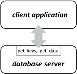
Figure 1: Block diagram of the interface. The interface

connects a client application with a server providing the

data through the functions get_keys and get_data.

A Generic Interface Speciﬁcation for Standardized Retrieval and Statistical Evaluation of Spatial and Temporal Data

137

function get_data. They effectively define the

vocabulary understood by the server. In trusted

computing environments one might consider adding

a clientID input parameter to get_keys in order to

provide different clients with different sets of

capabilities. In untrusted environments one should

rather resort to more reliable authentication methods

though.

2.1 list_of_functions

The list_of_functions returned by get_keys contains

a list of all supported scalar aggregation functions

–at least one– that the server can apply to each group

of selected data (as explained further below). In

particular, statistical functions can be applied. For

example,

• “mean” – the arithmetic mean,

• “SD” – the (corrected) sample standard

deviation,

• “n” – the number of selected/aggregated

elements,

and for robust statistics and box plots:

• “median” – the median,

• “Q1”, ”Q3” – the first and third quartile,

• “min”, “max” – the minimum and maximum.

Vice versa, the list_of_functions provided as a

parameter to get_data can be a (non-empty) list of

any of these elements. A corresponding number of

results will be returned accordingly, as shown

further below.

2.2 list_of_measurement_quantities

The list_of_measurement_quantities returned by

get_keys consists of a list of associative arrays. Each

array in that list contains the metadata of a particular

scalar measurement quantity that can be queried in

the database of the server. The metadata is given in

terms of a number of (key, value)-pairs and specific

text strings are used as keys. A mandatory (key,

value)-pair is the (“identifier”, measurement_

identifier)-pair. The measurement_identifier can be a

number or a string that uniquely identifies an

accessible measurement quantity in the database

comprising a multitude of scalar measurements in

space and time. Each individual measurement should

be associated with a timestamp and a spatial location

(e.g., latitude longitude, and elevation). In case of

missing timestamps, the affected measurements

should be ignored when temporal constraints are

specified in a query. In case of missing location

information, the affected measurements should be

ignored when spatial constraints are given. In other

words, constraints are considered unfulfilled if the

respective information is missing.

To give an example, a measurement_identifier

could be given in the form of a text string like this:

“BikeSharingCompanies(Company1).NumberOf

AvailableBikes“.

This identifier would be associated with

measurements of the number of available bikes in all

bike sharing stations of a particular bike sharing

company.

The list_of_measurement_identifiers provided as

a parameter to get_data is a (non-empty) list of

these measurement_identifiers. A corresponding

number of results with regard to the respective

measurement quantities will be returned in the

corresponding order, as shown in detail further

below.

Besides this essential (key, value)-pair, other

metadata information about a measurement quantity

might be required, e.g.,

• “locations” (key) – value: a list of all existing

measurement locations for the given quantity.

Each element in the list may contain the specific

coordinates and/or a string with the name of the

location. This allows the client to query data

from specific locations (in get_data). In the bike

sharing example, these could be locations of

particular bike sharing stations.

• “areas” – a list of spatial areas where the data is

measured. An area can be specified, for example,

as a polygon on a two-dimensional surface

and/or by a name given in a string. This provides

the client with another possibility to filter data

spatially.

• “measured since” – timestamp of the first

available measurement. Such a timestamp can be

specified as appropriate, typically as RFC 3339

or ISO 8601 timestamp.

• “measured until” – timestamp of the last

available measurement. A special indicator

timestamp can be defined to designate ongoing

measurements.

• “name” – a string containing the (human-

readable) name of the measured quantity, e.g.,

“number of available bikes”.

• “unit” – a string containing the unit of the

measured quantity, e.g., an SI unit like “kg” or

“m”. Measurement quantities without unit (e.g.

“number of available bikes”) can be denoted

with an empty string.

Categorical quantities: A special case can be

introduced to enable the processing of

KMIS 2015 - 7th International Conference on Knowledge Management and Information Sharing

138

measurements of categorical variables with this

interface. For this purpose, the value of “unit”

can be given as a list of strings, each string

denoting a category, e.g., “red”, “green”, and

“blue”. The measurement of a categorical

variable can then be represented in terms of

scalar numbers (hence fitting into the given

framework), each number constituting the

ordinal number of a category in the list of

category names. Note, however, that it generally

does not make sense to use aggregation functions

like “mean” and “median” in conjunction with

ordinal numbers. Therefore, the access to

categorical data is mainly confined to the use of

the function “n” in combination with the filter

condition “value_is” (see below).

• “description” – a string that contains a textual

description of the measured quantity.

Other (key, value)-pairs of metadata can be added, if

necessary.

2.3 list_of_condition_keywords

The list_of_condition_keywords returned by

get_keys contains a list of all supported keywords

that can be used to define filters for the selection of

measurements to be aggregated and retrieved. The

precise use of the keywords is explained in section

2.5, in this section we provide a condensed overview

of the different types of filters. The first type of

these filters selects measurements from particular

time intervals. Such filters can be, e.g.,

• “time_of_day” – to specify a time interval within

a day

• “day_of_week” – to specify a range of week

days, e.g., Mon-Fri

• “day_of_month” – to specify a range days within

a month, e.g., 1.-15.

• “week_of_year” – to specify a range of calendar

weeks

• “month_of_year” – to specify a range of months

within a year

• “year” – to specify a range of years

• “last_n_days”

Special keywords are

• “continuous_binning” – to specify a series of

time intervals

• “all” – to impose no restrictions

The second type of filter restricts the selection of

measurements spatially, e.g.:

• “within_distance_of” – to select measurements

•

within a certain distance from a given spatial

location

• “within_area_of” – to select measurements

within a certain area

The third type of filter is a restriction with respect to

the values of the measurements:

• “value_within” – to select measurements whose

value is within a certain range

• “value_is” – to select measurements with a

particular value

Finally, there is a more complex fourth type of filter

that conditions the selection of each measurement on

measurement results of another measurement

quantity:

• “corresponding_attribute”

• “corresponding_temporal_attribute”

• “corresponding_spatial_attribute”

• “corresponding_spatiotemporal_attribute”

The next sections explain how to use these

keywords.

2.4 list_of_conditions

Each of the three last parameters of get_data,

(list_of_conditions0, list_of_conditions1, and

list_of_conditions2) contains a list of freely

combinable conditions.

For each measurement quantity requested by

get_data in the list_of_measurement_identifiers,

each measurement associated with that measurement

quantity is aggregated in a cell of a two-dimensional

table, if it fulfils particular conditions given in the

three lists of conditions. First of all, all conditions

given in the list_of_conditions0 must be met (the

“global” conditions). Second, if the mth condition in

list_of_conditions1 and the nth condition in

list_of_conditions2 are fulfilled, then the

measurement is assigned to the mth row and nth

column of the table (the “local” conditions).

Measurements can be assigned to more than one

cell of the table, if they fulfil more than one pair of

conditions in list_of_conditions1 and list_of_

conditions2. After all measurements have been

checked and possibly assigned to a cell, each set of

measurements (given in each cell) is processed by

all aggregation functions specified in

list_of_functions. In effect, a scalar result is obtained

for each function in list_of_functions and each cell

of the table and each measurement quantity in the

list_of_measurement_identifiers, making up a four-

dimensional array_of_scalars returned by get_data.

If the set of measurements in a cell of the

aggregation table is empty, most aggregation

A Generic Interface Speciﬁcation for Standardized Retrieval and Statistical Evaluation of Spatial and Temporal Data

139

functions are undefined and the array_of_scalars

should reasonably contain a NaN (“not a number”,

IEEE 754 floating-point standard used for missing

values) at the corresponding position (or an

equivalent value, if NaN is not supported). One

exception is the counting function “n”, which returns

a zero in this case. Another special case is the

corrected sample standard deviation, “SD”, which is

undefined also for a single measurement. In this

case, one could either consistently return a NaN or

revert to the uncorrected sample standard deviation,

which is zero in this case.

2.5 Conditions

Each individual condition can be either true or false

with respect to a single scalar measurement. It

consists of a keyword from the

list_of_condition_keywords supplemented with a

certain number of parameters. We use the following

syntax for such parameterized keywords:

condition_keyword(parameter1, parameter2, …,

parameterN)

Irrespective of this, depending on the particular

implementation, one might as well resort to other

syntactical formulations.

2.5.1 Temporal Constraints

Conditions related to the time of the measurements

will mostly have one or two parameters, specifying a

point in time or a time range, e.g.

• “time_of_day(10:00, 12:00)” – to select data

measured between 10 and 12. More precisely, all

data measured at times t fulfilling the condition

10:00 ≤ t < 12:00. Note that t=12:00 is excluded

here to prevent the same data appearing twice in

selections like “time_of_day(10:00, 12:00)” and

“time_of_day(12:00, 14:00)”.

• “time_of_day(10:00)” - to select data from a

single point in time, here 10:00.

Similarly, “day_of_week(Mon, Fri)” would restrict

data to be chosen between Monday and Friday and

“day_of_week(Mon)” would restrict data to be

chosen from Monday only. In all cases except

“time_of_day”, the second argument is meant to be

inclusive, e.g. “year(2012, 2014)” selects data from

years 2012, 2013, and 2014. Accordingly, the filters

“day_of_month”, “week_of_year”, and “month_of_

year” can take one or two integers as parameters,

whereas the filter “last_n_days” has only one

(positive) integer as parameter.

As an alternative, in accordance with ISO 8601,

one might consider defining also all times uniformly

in terms of single numbers: time in the format

HH:MM could be defined as HHMM (or

HH:MM:SS as HHMMSS). The days of the week

could be enumerated from 1 (Monday) to 7

(Sunday).

The following conditions implement special

functions:

• “continuous_binning(start_time, time_ interval,

end_time)” – this specifies a whole list of

consecutive time intervals of length

time_interval (in seconds), starting at a given

point in time, start_time, and ending at end_time.

These timestamps can be specified, e.g.,

according to RFC 3339 or ISO 8601, as already

suggested in section 2.2. Recommended is the

use of “continuous_binning” as sole element in

either list_of_conditions1 or list_of_conditions2.

It is useless in list_of_conditions0 (where it

should be evaluated consistently as an

unfulfillable condition). Aside from statistical

assess-ments, continuous binning can be used

with “mean” or “median” to equidistantly (sub-

)sample the measurement data and thus to obtain

a regularized representation of the data.

• “all” – always fulfilled, to impose no restrictions

(has no parameters).

2.5.2 Spatial Constraints

Conditions related to the location of the

measurements can be defined, e.g., as follows

• “within_distance_of(location, 0, 20)” – to select

data measured at a distance between 0 and 20

meters of a certain location. A location can be

specified as appropriate, for example as

Cartesian coordinates or in terms of latitude,

longitude, and elevation. Alternatively, the server

could also provide a list of names (text strings)

defining particular locations of interest in the

“locations” (key, value)-pair, each name being

accepted as a valid location in

“within_distance_of”.

• “within_area_of(area)” – to select data measured

within a defined area. As stated in section 2.2, an

area can be specified, for example, as a polygon

on a two-dimen-sional surface or just by a name

(text string) provided in the “areas” (key, value)-

pair, implicitly defining a particular area of

interest.

KMIS 2015 - 7th International Conference on Knowledge Management and Information Sharing

140

2.5.3 Constraints Regarding the

Measurement Value

Conditions related to the measured value itself can

be defined, e.g., as follows

• “value_within(-0.5, 1)” – to select measurement

data with values between -0.5 and 1.

• “value_is(-0.5)” – to select measurement data

with a value of -0.5.

Note that these constraints apply to all

measurement quantities requested in get_data.

Therefore, if multiple measurement quantities are

requested in conjunction with value constraints, the

measurement quantities should usually be of the

same type.

2.5.4 Constraints with Respect to Another

Measurement Quantity

Sometimes it is necessary to select data depending

on the state of a different measurement quantity. For

example, the number of bicycles in use will probably

depend on the weather. To facilitate evaluations in

this respect, the following conditions are proposed:

• “corresponding_attribute(identifier, mode, min,

max)” – the basic condition.

All measurement values of the (other) quantity,

specified by the identifier, are processed

according to a given mode taking one of the

following values:

- “mean”, the mean of all measurements is

considered,

- “median”, the median of all measurements is

considered,

- “exists”, to verify if at least one measurement

fulfils the condition,

- “all”, to verify if all measurements fulfil the

condition,

- “closest_in_time”, only the measurement with

the smallest absolute time difference to the

measurement of the primary measurement

quantity is considered,

- “closest_in_space”, only the measurement with

the smallest spatial distance to the measurement

of the primary measurement quantity is

considered.

The condition is fulfilled if the considered value

is between min and max, i.e. min ≤ value ≤ max.

If there is no measurement, the condition is not

fulfilled.

• “corresponding_temporal_attribute(identifier,

mode, min, max, t_min, t_max)” – extends the

basic condition with a time constraint. Each

measurement of the corresponding measurement

quantity is considered only if the difference in

time between the measurement of the primary

measurement quantity and the measurement of

the corresponding measurement quantity lies

within a certain range [t_min, t_max]. Each

parameter, t_min and t_max, denotes a time

difference in seconds, which can also be a

negative value.

• “corresponding_spatial_attribute(identifier,

mode, min, max, d_min, d_max)” – extends the

basic condition with a spatial constraint. Each

measurement of the corresponding measurement

quantity is considered only if the spatial distance

between the measurement of the primary

measurement quantity and the measurement of

the corresponding measurement quantity lies

within a certain range [d_min, d_max]. Each

parameter, d_min and d_max, denotes a distance

in meters.

• “corresponding_spatiotemporal_attribute(identifi

er, mode, min, max, d_min, d_max, t_min,

t_max)” – extends the basic condition with a

spatial and a temporal constraint. Each

measurement of the corresponding measurement

quantity is considered only if (a) the spatial

distance between the measurement of the

primary measurement quantity and the

measurement of the corresponding measurement

quantity lies within a certain range [d_min,

d_max], and (b) the difference in measurement

time lies within a certain range [t_min, t_max].

The parameters d_min and d_max denote a

distance in meters and the parameters t_min and

t_max denote a time difference in seconds.

2.6 A Simple Example using Lists of

Conditions

The list_of_conditions1 and list_of_conditions2 are

of the same type, but will usually contain different

lists of conditions. As an example,

list_of_conditions1 might contain

[“day_of_week(Mon)”,

“day_of_week(Tue)”,

“day_of_week(Wed)”]

and list_of_conditions2 might contain

[“time_of_day(10:00,12:00)”,

“time_of_day(12:00,14:00)”,

“time_of_day(14:00,16:00)”],

resulting in a table with 3×3 entries of aggregated

data (for each measurement quantity specified in

A Generic Interface Speciﬁcation for Standardized Retrieval and Statistical Evaluation of Spatial and Temporal Data

141

list_of_measurement_identifiers and each aggre-

gation function specified in list_of_functions).

Table 1: Example of a table containing aggregated data.

The matching data varies among the cells of the table and

depends on the respective conditions for each row and

each column.

Measu-

rement

quantity

10:00-12:00 12:00-14:00 14:00-16:00

Mon

mean(matching

data),

median(matching

data),

…

mean(matching

data),

median(matching

data),

…

mean(matching

data),

median(matchin

g data),

…

Tue

mean(matching

data),

median(matching

data),

…

mean(matching

data),

median(matching

data),

…

mean(matching

data),

median(matchin

g data),

…

Wed

mean(matching

data),

median(matching

data),

…

mean(matching

data),

median(matching

data),

…

mean(matching

data),

median(matchin

g data),

…

The list_of_conditions0 contains a list of global

constraints that apply to the overall table in addition

to the constraints previously defined for the columns

and rows of the table. As an example, this could be

[“year(2001,2010)”, “month_of_year(1)”] to get

some statistics averaged over all Januaries from

2001 till 2010.

2.7 array_of_scalars

The array_of_scalars returned by get_data is a

four-dimensional array of floating point numbers.

The array is of the size k×l×m×n corresponding to

• k aggregation functions specified in

list_of_functions,

• l scalar measurement quantities specified in

list_of_measurement_identifiers,

• m conditions specified in list_of_conditions1,

• n conditions specified in list_of_conditions2.

Each element in the array contains the result of the

corresponding aggregation function applied to those

measurements of the respective measurement

quantity that match the corresponding conditions:

single_element = array_of_scalars[g][h][i][j],

in which g refers to the gth function in

list_of_functions, h refers to the hth measurement

quantity in list_of_measurement_identifiers, i refers

to the ith condition in list_of_conditions1, and j

refers to the jth condition in list_of_conditions2.

For example, with a single call to get_data one

can obtain the mean and standard deviation

(list_of_functions) of the number of available

bicycles, individually for a number of bike sharing

companies (list_of_measurement_identifiers) and

separately for each hour of the day

(list_of_conditions1) and each day of the week

(list_of_conditions2). These statistics can be limited,

for example, to a certain time span, like “all

Januaries from 2001 till 2010” (list_of_conditions0).

It is, of course, conceivable to extend the table

spawned by list_of_conditions1 and

list_of_conditions2 to more dimensions by adding

lists of conditions as additional parameters to

get_data. However, the use of two-dimensional

tables is often the most convenient option, in

particular for visualizations of the obtained statistics.

3 CONCLUSIONS

We presented a generic interface specification for

standardized retrieval and statistical evaluation of

spatial and temporal measurement data provided by

a software service. The two functions of the

interface can be implemented as remote procedure

calls (RPC) to the service. For example, one possible

realization would be the use of HTTP-based calls

over the Internet. The interface is not specific to a

particular type of database, programming language,

or data format. It also does not demand a specific

syntax nor is the scope of its functionality

completely fixed. In this way, it allows for an easy

adaptation to the specific needs and requirements of

a particular software implementation. In contrast to

the standards developed by OGC and ISO TC/211,

the proposed specification is much leaner and

features an efficient statistical aggregation of the

data on the server side, thereby minimizing the

amount of data to be transferred to the client.

On the other hand it should be noted that the

presented specification is restricted to the retrieval of

numerical data, whereas the OGC and ISO standards

have a much broader scope. It therefore would be

beneficial if the OGC and the ISO TC/211 could

consider including similar statistical aggregation

functionality into their standards in the future. Also,

the specific filters that we proposed in section 2.5.4

to select data according to the state of another

quantity may be adopted in OGC filters by

implementing user-defined functions according to

the definitions in 2.5.4.

We will implement the presented interface in a

mobility management platform for smart cities. A

KMIS 2015 - 7th International Conference on Knowledge Management and Information Sharing

142

client application, the so-called mobility

management and emission control panel, will

analyse and visualize all data collected on a central

mobility data integration platform. Access to the

data will be performed by using the proposed

interface and HTTP-based calls.

ACKNOWLEDGEMENT

The research leading to these results has received

funding from the European Union Seventh

Framework Programme (FP7/2007-2013) under

grant agreement n° 608991, project STREETLIFE.

REFERENCES

http://www.opengeospatial.org

http://www.isotc211.org

http://www.isotc211.org/Outreach/Overview/

Overview.htm

Alonso, G., Casati, F., Kuno, H., Machiraju, V., 2004.

Web Services. Springer Berlin Heidelberg.

Erl, T., 2005. Service-oriented architecture: concepts,

technology, and design. Pearson Education.

Snodgrass, R.T., et al., 1995. The TSQL2 Temporal Query

Language. Kluwer Academic Publishers.

Egenhofer, M. J., 1994. Spatial SQL: A Query and

Presentation Language. In IEEE Transactions on

Knowledge and Data Engineering, 6(1):86–95.

Chen, C.X., Zaniolo, C., 2000. SQL

: A Spatio-Temporal

Data Model and Query Language. In Proceedings of

the 19th International Conference on Conceptual

Modeling, pp. 96-111.

Erwig, M., Schneider, M., 2002. STQL: A Spatio-

Temporal Query Language. In Mining Spatio-

Temporal Information Systems (eds. R. Ladner, K.

Shaw, and M. Abdelguerfi), Kluwer Academic

Publishers, pp. 105-126.

http://www.opengeospatial.org/standards/filter

A Generic Interface Speciﬁcation for Standardized Retrieval and Statistical Evaluation of Spatial and Temporal Data

143