Using Collective Intelligence to Generate Trend-based Travel
Recommendations
Sabine Schlick, Isabella Eigner and Alex Fechner
Institute of Information Systems, Friedrich-Alexander University, Lange Gasse 20, 90403, Nürnberg, Germany
Keywords: Trend-based Recommender System, Spatio-Temporal Travel Trends, Individualized Travel
Recommendations, Collective Intelligence.
Abstract: Trips are multifaceted, complex products which cannot be tested in advance due to their geographical distance.
Hence, making a travel decision people often ask others for advice. This leads to an increasing importance of
communities. Within communities people share their experiences, which results in new, more extensive
knowledge beyond the individual knowledge of each member. The objective of this paper is to use this
knowledge by developing an algorithm that automatically generates trend-based travel recommendations.
Based on the travel experiences of the community members, interesting travel areas are identified. Five key
figures to evaluate these areas according to general criteria and the users’ individual preferences are
developed. The algorithm allows to generate recommendations for the whole community and not only for
highly active members, resulting in a high coverage. A study conducted within an online travel community
shows that automatically generated, trend-based trip recommendations are rated better than user-generated
recommendations.
1 INTRODUCTION
Trips are multifaceted, complex products that consist
of many different components. Due to their
geographical distance they cannot be tested in advance
(Hwang, Gretzel and Fesenmaier, 2002). When it
comes to travel decisions, people are highly motivated
to exchange experiences with others. This emphasizes
the important role of communities in tourism, as they
often provide better support in information search than
guidebooks (Prestipino and Schwabe, 2005). Research
even shows that recommendations from users are
rated better than automatically generated
recommendations (Magno and Sable, 2008).
Exchanging their experiences within online-
communities, people generate new knowledge beyond
the knowledge of the individuals (Bächle, 2008).
Whereas the members of a travel community have
knowledge about single trips they did in the past and
can share their experiences, the collected knowledge
of all community members is much more extensive.
This phenomenon is defined as collective intelligence
(Malone, Laubacher and Dellarocas, 2009). By
analyzing this knowledge, new, enriched knowledge
can be generated (Gruber, 2008). On the downside,
the increasing amount of user-generated content leads
to an information overload for the users (Jannach,
2011). Recommender systems tackle this problem by
suggesting products that fit the individual preferences
of the customers (Smyth, 2007). Besides content-
based and collaborative filtering, the two classical
approaches, demography-based, knowledge-based,
utility-based and hybrid methods exist (Burke, 2002).
Moreover, other recommender systems are based on
social relationships and trust between users (Meo et
al., 2011). Overall measures for the quality of
recommender systems are the quality of the
recommendation (the rating of the users) and the
coverage (percentage of users a recommendation can
be generated for) (Massa and Avesani, 2007).
The goal of this paper is to use the collective
knowledge of a travel community to generate
individualized, trend-based travel recommendations.
By analyzing the places community members have
visited in the past, relevant travel areas are detected.
Based on these travel areas, individualized
recommendations of trips within these travel areas are
generated. We then evaluate if the automatically
generated, trend-based recommendations are rated
better than the trips recommended by the members of
the community while increasing the coverage.
This paper is structured as follows. Chapter 2
gives an overview of related work followed by the
Schlick, S., Eigner, I. and Fechner, A..
Using Collective Intelligence to Generate Trend-based Travel Recommendations.
In Proceedings of the 7th International Joint Conference on Knowledge Discovery, Knowledge Engineering and Knowledge Management (IC3K 2015) - Volume 1: KDIR, pages 177-185
ISBN: 978-989-758-158-8
Copyright
c
2015 by SCITEPRESS – Science and Technology Publications, Lda. All rights reserved
177
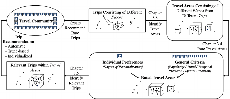
Figure 1: Approach.
method development and the single steps of the
algorithm (chapter 3). Chapter 4 deals with the study
to evaluate the trend-based recommendations. Chapter
5 summarizes the findings, outlines limitations, and
gives suggestions for future research.
2 RELATED WORK
Many recommender systems either integrate user
preferences or spatio-temporal trends in the
recommendation process. Wallace et al. (2004) and
Ricci et al. (2006) use product bundles and travel
plans of other users to generate recommendations,
whereas Gruber (2008) and Frers (2010) integrate
user knowledge about travel destinations. While the
focus of these systems lies on the matching of user
preferences and trip characteristics, spatio-temporal
factors are only considered as trip characteristics.
In contrast, others focus on spatial and temporal
aspects as an influencing factor for their
recommendations. The hybrid system of Sebastia et
al. (2009) not only bundles places, but orders them
chronologically. Others also consider temporal
factors to analyze the availability of single points of
interest (Tung and Soo, 2004). While Baraglia et al.
(2012) only use spatial data to find suitable travel
routes, Monreale et al. (2009) additionally extract the
spent time within user trajectories to find common
paths. Yoon et al. (2012) also utilize user trajectories
to group single places to interesting travel regions, but
disregard the temporal development of the popularity.
Existing approaches show the high relevance of
spatio-temporal data for travel recommendations.
However, the detection of both spatio-temporal trends
in combination with further personalization is not
considered yet. By exploiting this gap, our new
approach enables users with low activity within the
community and thus limited information to also
receive valuable recommendations. Personalized
recommendations for active community members can
also be improved by considering general travel trends
for more diversified suggestions.
3 METHOD DEVELOPMENT
3.1 Approach
To develop an algorithm to automatically generate
trend-based recommendations, this research follows
the design science paradigm (Hevner et al., 2004).
Figure 1 gives an overview on the developed
approach. Starting point is a travel platform that
enables users to create trips consisting of individual
places. The trips as well as the single places comprise
a number of attributes, e.g. the location type. Within
this travel community, users share and rate their travel
experiences or recommend trips to other users.
According to the theory of collective intelligence
(Malone, Laubacher and Dellarocas, 2009), new
knowledge that is more extensive than that of the
single community members, emerges. By analyzing
this collective knowledge, new, enriched knowledge
about travel trends and user preferences can be gained.
First, the places users visited in the past are analyzed
to identify relevant travel areas. As a next step,
criteria to rate these travel areas are developed.
KDIR 2015 - 7th International Conference on Knowledge Discovery and Information Retrieval
178
General criteria as well as the fit of a travel area to the
individual user preferences are taken into account.
Afterwards, relevant trips for the individual users
within these travel areas are identified and
recommended to the community members. To
evaluate the findings, user ratings for the
automatically generated recommendations are
compared to user-generated recommendations.
3.2 Data Set
User-generated content is used to identify travel areas
and to provide the recommendations. On the travel
platform users create trips consisting of one or more
places they have visited by tagging the single places
on a map. The geo-coordinates are assigned
automatically. Users add some characteristics from a
predefined selection to the trips and places.
Characteristics of trips are the date (from-to), the
travel style (e.g. couple), and the travel type (e.g.
cruise). Characteristics of the places are the location
type (e.g. beach), the transportation (e.g. by car), the
activities (e.g. swimming), and the costs (in Euro).
3.3 Identify Travel Areas
Based on the places users create on the travel
platform, travel areas, defined as an accumulation of
places, have to be identified. Neither the spatio-
temporal location nor their extent is known in
advance. The spatial extent of a travel area is e.g. a
certain city or region. Besides the spatial extent, the
temporal extent plays an important role. A skiing
region in the Alps can be popular in winter, but is also
visited in summer for hiking activities. The skiing
region in winter might be smaller than the hiking
region in summer, but might have more visitors.
Therefore, two travel areas have to be identified.
Using the user-generated content the algorithm is able
to detect the relevant spatial and temporal extent for
each travel area. To find travel areas, places that are
nearby in spatial and temporal respect have to be
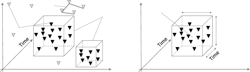
detected. Figure 2 shows places (triangles), trips
(bundles of places), and two accumulations of places
(boxes) that define travel areas (left hand side). Based
on this accumulation of places, the position and the
extent of a travel area can be detected. The position is
defined by the spatial (longitude and latitude) and the
temporal (time) position (right hand side). The extent
is determined by the spatial and the temporal distance
between the position and the places with the highest
spatial and temporal distance.
To identify travel areas, the “Density–Based
Spatial Clustering of Applications with Noise
(DBSCAN)” algorithm is applied (Ester et al., 1996).
This algorithm allows to identify clusters even if
neither the number of clusters nor their extent and
shape is known. If the distance of two objects is below
a certain threshold ε, these objects are neighbors.
Objects (places) are assigned to a cluster (travel area)
if they have a minimal number of dense neighbors or
if they are dense to an object that has a minimal
number of dense neighbors, otherwise they are noise.
Since the DBSCAN only uses one threshold for
clustering, the algorithm has to be adapted in a similar
way as proposed by Birant and Kut (2007). They
adapted the DBSCAN to cluster objects in spatial,
temporal and non-spatial respect. To detect travel
areas, only spatial and temporal aspects are relevant.
Therefore, two thresholds are taken into account, a
spatial threshold ε
and a temporal threshold ε
, that
amount to the spatio-temporal threshold ε
=
(
ε
,ε
)
. An object is only assigned to a cluster, if the
spatial and the temporal distances are lower than the
spatial and the temporal thresholds. Two places
(
p
,p
)
are neighbors if their spatial and temporal
distances
are smaller than the given spatio-
temporal threshold:
(
,
)
≤
(1)
Figure 2: Places, trips, and spatio-temporal travel areas.
Latitude
Longitude
Latitude
Longitude
Places
Travel areas
Longitude
Latitude
x
Position
Trip
Using Collective Intelligence to Generate Trend-based Travel Recommendations
179
The spatial and the temporal distance have to be
calculated separately. Spatial places
are described
by their geographical coordinates, the latitude , the
longitude and the constant radius of the earth R,
= (,,) (Nitschke, 2014). A spatio-temporal
place is additionally defined by its point of time t,
= (,,,). The spatio-temporal distance is
calculated by the vector over the spatial distance
and the temporal distance
:
,
=
,
,
(2)
To calculate small spatial distances between two
places the Haversine formula (Sinnott, 1984) is
considered to be very suitable (Montavont and Noel,
2006). As travel areas consist of a number of close
places, the distances thus are by definition small. The
temporal distance is calculated by the difference
between two points of time t
1
and t
2
. Applying the
cluster algorithm, spatio-temporal accumulations of
places are detected. Knowing the places of a certain
travel area, the position
is calculated. It is defined
by the temporal and the spatial center. The temporal
center
is computed, which requires the arithmetic
mean of the points in time. To identify the spatial
center, the geographical coordinates first have to be
converted into Cartesian coordinates. After
calculating their arithmetic mean they are
transformed back into geographical coordinates
(Nitschke, 2014). Subsequently, the spatio-temporal
extent
=
(
,
)
is calculated. The spatial extent
is the geographical distance
(
,
)
between the position
of the travel area and the
place within this travel area that has the highest
distance to the position
. Analogously, the place
that has the highest temporal distance to the
position of a travel area is used to compute the
temporal extent
(
,
)
. In conclusion, a
travel area can be described by its position and its
spatial and temporal extent =(
,
,
).
3.4 Rate Travel Areas
After the identification of travel areas in general, five
key figures to rate these travel areas are developed.
Four of these key figures (popularity, trend, spatial
precision and temporal precision) are general criteria
and used for the whole community. To consider
individual preferences of the single users, a fifth key
figure (degree of personalization) is introduced.
3.4.1 General Criteria
Popularity: The popularity is measured by the
number of visitors. The more users visit places in a
certain travel area the higher is the popularity of that
travel area:
=
(3)
Trend: Using only the number of visitors in a
certain area is not sufficient. Travel areas that have a
high number of visitors might be identified as
relevant areas, even if the number of visitors is
strongly decreasing over time. Besides, upcoming
relevant trend areas might not be recognized.
Therefore, a second key figure is introduced to
observe the popularity of the travel areas over time.
The challenge is to identify a certain travel area in
different time periods, e.g. years, because travel areas
will not have the exact same position and extent each
period as new places might be added or others
disregarded. Therefore, travel areas that are
equivalent to each other in different time periods are
identified by using the similarity of their positions
and their extents. The higher the similarity, the higher
the probability that two travel areas are equivalent.
The initial requirement for two travel areas to have a
similar position is to be adjacent. In other words, the
distance between the positions of two areas has to be
equal or lower than the sum of their extents. Hence, a
flexibly adaptable threshold is introduced, that is
dependent on the extent of the travel areas. With
travel areas that have a small extent, like a small
festival, the threshold is lower than the one for travel
areas with a larger spatial and temporal extent, e.g. a
hiking area. If the distance of the positions is lower
than this threshold, the travel areas are equivalent.
The threshold is defined by the spatio-temporal extent
of the considered travel area
and the
potentially equivalent travel area
:
ℎℎ=e
ta
+e
ta
(4)
All potentially equivalent travel areas
that
have a lower distance to the considered travel area
than the individual threshold, are so called
candidates
. Figure 3 illustrates on the left hand
side travel areas with different extents. On the right
hand side, overlapping travel areas are shown. The
distance between the positions a and b is smaller than
the threshold: they overlap. The distance between b
and c and a and c is higher than the threshold. They
are not overlapping or adjacent.
After generating a list of candidates for each travel
area, the extent of a travel area is taken into account.
The more similar the extent of the considered travel
area
and a candidate
, the higher the
KDIR 2015 - 7th International Conference on Knowledge Discovery and Information Retrieval
180

Figure 3: Using the position of travel areas to identify equivalent travel areas.
probability that they represent the same travel area in
different time periods. Therefore, the Euclidian
distance between the extent of the considered travel
area
and the candidate
is used. The
candidate with the lowest distance is identified as the
equivalent travel area to the considered travel area.
Having identified equivalent travel areas, the
development of the number of visitors can be
observed. Therefor the linear regression is applied to
measure if the number of visitors (dependent
variable) is increasing (positive algebraic sign) or
decreasing (negative algebraic sign) over multiple
time periods (
) (independent variable). The value of
the regression coefficient expresses the strength of the
connectivity. Referring to (Bortz and Schuster, 2010),
the second key figure (trend) is calculated as follows:
=
∑(
)
(
)
∑(
)
(5)
Spatial and Temporal Precision: The next two
key figures concentrate on the characteristics of these
travel areas. The number of places within a travel area
and the number of their assigned characteristics is
different for all areas. To overcome this issue, a
weight for each characteristic
is calculated for
all travel areas. The more often a characteristic occurs
in a certain travel area, the higher the importance of
this characteristic. The weight for a characteristic is
the occurrence frequency divided by the number of
placesin a certain travel area. Travel areas that have
a big local and global extent, but a low number of
places, may be described worse by their
characteristics than small travel areas with a high
number of places. The spatial and the temporal
precision thus describe the accuracy of the
assignment of the characteristic attributes. They are
calculated by the popularity divided by the spatial and
the temporal extent, respectively:
=
=
(6)
3.4.2 Individual Preferences
Degree of Personalization: So far, travel areas can be
rated by general criteria. However, users differ in
their preferences (Zins and Grabler, 2006). By
considering individual preferences in addition to
general criteria, customized recommendations can be
given to each user. As users are assumed to like what
they liked in the past (Adomavicius and Tuzhilin,
2005), trips and places they created and rated well are
used to identify their preferred trip characteristics.
These characteristics may include attributes
describing the entire trip (e.g. travel type) or specific
details of the single places (e.g. activities).
Users that highly favor a certain characteristic will
have visited many places containing this
characteristic. The more often it can be found in the
places a user visited, the more relevant this attribute
is for the considered user. Analogously to the weights
for the travel areas, weights of the preferred attributes
of a user
are calculated, by dividing the
occurrence frequency of the attributes by the number
of places visited by the user. By calculating the
Euclidian distance between the weight of the
describing attributes of a travel area and the weight of
the preferences of the user the degree of
personalization can be determined. This key figure
states to which degree a considered travel area fits the
preferences of a user. The lower the value of the key
figure, the better the travel area fits:
=
∑
−
(7)
Latitude
Longitude
Latitude
Longitude
x
x
a
c
b
x
x
x
x
x
Using Collective Intelligence to Generate Trend-based Travel Recommendations
181

3.4.3 Apply Key Figures
All in all, five key figures to evaluate travel areas are
developed, the popularity, the trend, the spatial
precision, the temporal precision, and the degree of
personalization. Whereas the first four key figures are
the same for all users, the last one has to be calculated
for each user separately. Applying the key figures, all
travel areas have to be evaluated in comparison to
each other. First all travel areas are ranked within the
single key figures. The travel areas with the best value
is ranked with one, the second best with two and so
on. Afterwards, an overall rating is calculated.
Therefore the single ranks of the key figures (
) for
each travel area are summed up and divided by the
number of key figures. To change the influence of a
single key figure, a weight (
) is introduced:
ng
(ta)=
∑
∗
(8)
Table 1 gives an example for different values (V)
for the five key figures and the assigned rank (R).
While travel area
has the highest popularity with
990 visitors, the trend is higher for travel area
. If
two travel areas have the same value for a certain key
figure, e. g. travel area
and
()
for the key
figure temporal precision, both are assigned to the
lower rank. After calculating the rating, travel area
with a value of 1.8 is identified as the most
relevant travel area, followed by travel area
(all
key figures are weighted with one). The rating for the
trips can also be generated if not all key figures are
available. This way, the algorithm can also be applied
if, due to the low activity of a new user, the degree of
personalization cannot be calculated.
3.5 Identify Relevant Trips
In a last step, interesting trips within the relevant
travel areas are identified. Thus trips are rated
depending on the rating of the travel areas their places
belong to. If a place is associated with several travel
areas, the rating of all these travel areas is assigned to
the place. The rating of a trip is calculated by the sum
of the ratings of travel areas the single places are
allocated to, divided by the number of travel areas the
places are assigned to.
(t) =
∑
(
)
(9)
Table 2 summarizes the steps of the algorithm, the
applied methods as well as the flexibly adaptable
measures and the respective output.
4 EVALUATION
Within two weeks in 2013, a study is conducted,
where 60 participants are asked to create, rate and
recommend trips to each other on a travel platform.
Combined with already existing trips that were
created by other community members before the
evaluation study, 3,927 trips are available on the
platform. Altogether, the trips are made up of 4,817
places. Based on this data, the developed
recommendation algorithm is applied. The temporal
threshold
(
)
is set to 150 days and the spatial
threshold
(
)
to one kilometer. The minimal number
of neighbors (MinPts) is set to two. Assuming an
equivalent importance of the single key figures, their
weighting is set as follows: the spatial and the
temporal precision is set to 0.5, the popularity and the
trend to 1. The only factor considering the personal
preferences, the degree of personalization, is
weighted with three to balance the impact of general
and individual criteria on the recommendations.
Besides these automatically generated
recommendations, users recommend trips to each
other manually. Community members have to rate the
received recommendations using stars (1=very bad -
5=very good) to determine the fit with their actual
preferences. Altogether the participants rate 298 trip
recommendations, of which 198 (66%) come from
other users, 100 (34%) are generated automatically
using the developed algorithm. In general,
automatically generated, trend-based
Table 1: Calculating the rating of travel areas.
Travel
Area
Popularity Trend
Spatial
Precision
Temporal
Precision
Degree of
Personalization
Rating(ta)
V R V R V R V R V R
990 1 0.6 2 0.2 4 0.1 4 0.1 1 (1+2+4+4+1):5=2.4
878 2 0.7 1 0.5 2 0.4 2 0.25 2 (2+1+2+2+2):5=1.8
…
… … … … … …
()
450 3 0.4 3 0.8 1 0.4 2 0.89 4 (3+3+1+2+4):5=2.6
89 4 -0.3 4 0.3 3 0.2 3 0.7 3 (4+4+3+3+3):5=3.4
KDIR 2015 - 7th International Conference on Knowledge Discovery and Information Retrieval
182

Table 2: Recommending trips based on interesting travel areas – overview.
Steps
Method Flexibly adaptable Output
Identify travel
areas
Spatio-temporal clustering
Spatial threshold
(
)
Temporal threshold (
)
Minimal number of dense
neighbors (MinPts)
Accumulations of
places = Travel areas
Rate travel areas
by general and
individual criteria
Ranking all travel areas
according to the key figures
(popularity, trend, spatial
precision, temporal precision
and personalization)
Weightings for the single
key figures (
)
Travel areas rated by
their relevance for an
average user and for
individual users
Identify relevant
trips within fitting
travel areas
Using the rating of the travel
areas trips have places in to
evaluate single trips
Single trips within
these travel areas
recommendations receive better ratings (3.85 ± 1.29)
than recommendations by users (3.02 ± 1.14). To
avoid coincidental results, a t-test (Bortz and
Schuster, 2010) is executed using two independent
samples. It results in the rejection of the related null
hypothesis (“There is no difference between the
rating of user-generated and automatically generated
recommendations”) with a significance level of p <
0.01. There is a highly significant difference between
the means of the two samples. Therefore it can be
proven that the system is able to generate travel
recommendations that are qualitatively better than
user-generated recommendations.
To evaluate different parameter weightings and to
compare the new algorithm to traditional
recommendation methods a second study with 51
participants is conducted in 2015. These participants
create 131 new trips. All in all 827 trips consisting out
of 1,325 places are available on the platform. Four
settings are chosen for evaluation: In the first setting
the popularity as well as the trend are set to 1/6, the
spatial and the temporal precision to 1/12. The degree
of personalization has the highest influence and is set
to 1/2. In the second setting the popularity and the
trend are set to 1/3 and the spatial as well as the
temporal precision to 1/6. To analyze the relevance of
the degree of personalization, the parameter is set to
0 to compare the results with setting one. Thus the
recommendations are only based on travel trends.
In the third and fourth setting traditional
recommendation methods are tested and evaluated. In
setting three, a content-based approach relying on
similar items (Adomavicius and Tuzhilin, 2005), thus
trips that are similar to a user’s past trips, is used for
recommendations. Setting four follows a social
recommender approach, thus the trips of friends are
used for recommendations. Social recommender
systems are a special type of collaborative filtering
that utilize the similarity of users for
recommendations (Adomavicius and Tuzhilin, 2005).
The similarity of users can be identified by analyzing
their relationship (Meo et al., 2011). Therefore the
trip preferences of the participants’ friends in the
community are used to identify relevant trips for the
individual users. Trips that are similar to trips of
friends are identified and recommended to the
participants.
All in all 41 participants generate trips and it is
possible to provide recommendations based on
setting 1 and 3. 36 of the participants rate the received
recommendations. 30 participants become friends
with other users and recommendations based on
setting 4 are possible. All of them rate the received
recommendations. As travel trends can be identified
without active participation of the single users,
recommendations based on setting 2 can be generated
for the entire study group. 37 participants also rate the
recommendations. Moreover 48 participants receive
recommendations by other community members and
37 rate these recommendations. The 30 participants
that occur in all groups are used for analysis. They
rate the recommendations as follows: setting 1 is
rated with 3.948 (± 0.578), setting 2 with 3.877 (±
0.614), setting 3 with 3.972 (± 0,650), and setting 4
with 4.009 (± 0.645). The recommendations they
received by other users are rated with 3.313 (± 1.17).
To identify statistically relevant findings a paired
t-test (Bortz and Schuster, 2010) is conducted. The
related null hypothesis is as follows: “There is no
difference between the rating of user-generated
recommendations and the four settings of
automatically generated recommendations”. There is
a statistically significant difference between all
automatically generated recommendations and the
rating for the recommendations by the participants.
With a significance level of p < 0.05 all automatically
generated recommendations are rated better than
user-generated recommendations. Within the
Using Collective Intelligence to Generate Trend-based Travel Recommendations
183
automatically generated recommendations there is
only one statically significant difference between
setting 2 and setting 4. Recommendations based on
the taste of the friends of a user are rated better than
recommendations only based on travel trends with a
significance level of p < 0.05. Nevertheless,
recommendations only based on travel trends can be
generated for all users thus reducing cold start
problems for new or inactive members.
Recommendations based on the taste of friends can
only be generated if a user becomes friends with other
users on the platform, thus reducing the coverage of
recommendations to only socially active users.
5 CONCLUSIONS
In this paper, an algorithm to generate trend-based
individualized travel recommendations is developed.
The algorithm identifies travel areas based on user-
generated trips consisting of different places. Five
key figures are developed to rate these travel areas
based on general and individual criteria. General
criteria are the popularity of a travel area, the trend
and the spatial and temporal precision. The degree of
personalization allows to rate the travel areas based
on individual preferences for each single user. The
weights for these criteria are flexibly adaptable. It is
also possible to generate recommendations for users
that did not take part in the community actively and
for whom it is therefore not possible to compute a
degree of personalization yet. This way, general
recommendations can be generated for all community
members resulting in full coverage. To evaluate the
quality of the recommendations two studies are
conducted. Findings show that automatically
generated trend-based recommendations are
evaluated significantly better. Currently the algorithm
only uses the similarity of trips and travel areas to
calculate the degree of personalization. Besides this
kind of content-based approach, future research
concentrates on analyzing different measures to
calculate the degree of personalization (e.g.
collaborative approaches). Moreover, although the
set values for the thresholds and weightings already
lead to good results, further settings have to be
evaluated. Within the single key figures other
methods for calculation should be considered in
further studies. For clustering travel areas, e.g.
hierarchical clustering and geodesic k-means should
be tested. To adjust for seasonal and transient
variations, polynomial regression should also be
considered for estimating the popularity of an area.
REFERENCES
Adomavicius, G., and Tuzhilin, A. “Toward the next
generation of recommender systems: a survey of the
state-of-the-art and possible extensions.” IEEE
Transactions on Knowledge and Data Engineering 17,
no. 6 (2005): 734–749.
Bächle, Michael. “Ökonomische Perspektiven des Web
2.0– Open Innovation, Social Commerce und
Enterprise 2.0.” WIRTSCHAFTSINFORMATIK 50, no.
2 (2008): 129–132.
Baraglia, Ranieri, Frattari, Claudio, Muntean, Cristina
Ioana, Nardini, Franco Maria, and Silvestri, Fabrizio.
“RecTour: A Recommender System for Tourists.” In
2012 IEEE/WIC/ACM International Joint Conferences
on Web Intelligence (WI) and Intelligent Agent
Technologies (IAT). Piscataway: IEEE, 2012.
Birant, Derya, and Kut, Alp. “ST-DBSCAN: An algorithm
for clustering spatial–temporal data.” Data &
Knowledge Engineering 60, no. 1 (2007): 208–221.
Bortz, Jürgen, and Schuster, Christof. Statistik für Human-
und Sozialwissenschaftler. 7th ed. Berlin: Springer,
2010.
Burke, Robin. “Hybrid Recommender Systems: Survey and
Experiments.” User Modeling and User-Adapted
Interaction, November 2002, pp. 331–370.
Ester, Martin, Kriegel, Hans-Peter, Sander, Jörg, and Xu,
Xiaowei. “A Density-Based Algorithm for Discovering
Clusters in Large Spatial Databases with Noise.” In
KDD-1996: Proceedings of the 2nd international
conference on knowledge discovery and data mining:
AAAI Press, 1996.
Frers, Uwe. “Facebook-Applications im Tourismus –
Casestudy „Gedankenreise“ des Reiseportals
TripsByTips.” In Social Web im Tourismus: Strategien-
Konzepte- Einsatzfelder, edited by Daniel
Amersdorffer, Florian Bauhuber, Roman Egger and
Jens Oellrich. Berlin, Heidelberg: Springer Berlin
Heidelberg, 2010.
Gruber, Tom. “Collective knowledge systems: Where the
Social Web meets the Semantic Web.” Web Semantics:
Science, Services and Agents on the World Wide Web 6,
no. 1 (2008): 4–13.
Hevner, Alan R., March, Salvatore T., Park, Jinsoo, and
Ram, Sudha. “Design Science in Information Systems
Research.” MIS Quarterly 28 (2004): 75–105.
Hwang, Yeong-Hyeon, Gretzel, Ulrike, and Fesenmaier,
Daniel R. “Behavioral Foundations for Human-Centric
Travel Decision-Aid Systems.” In Information and
Communication Technologies in Tourism 2002:
Proceedings of the International Conference in
Innsbruck, Austria, 2002. Vienna: Springer Vienna,
2002.
Jannach, Dietmar. Recommender systems: An introduction.
New York: Cambridge University Press, 2011.
Magno, Terence, and Sable, Carl. “A Comparison of
Signal-Based Music Recommendation to Genre Labels,
Collaborative Filtering, Musicological Analysis,
Human Recommendation, and Random Baseline.” In
ISMIR 2008: Proceedings of the 9th International
KDIR 2015 - 7th International Conference on Knowledge Discovery and Information Retrieval
184
Conference of Music Information Retrieval, edited by
Juan Pablo Bello, Elaine Chew and Douglas Turnbull.
Philadelphia Drexel University, 2008.
Malone, Thomas W., Laubacher, Robert, and Dellarocas,
Chrysanthoas. “Harnessing Crowds: Mapping the
Genome of Collective Intelligence.” MIT Sloan
Research Paper No. 4732-09, 2009.
Massa, Paolo, and Avesani, Paolo. “Trust-aware
recommender systems.” In RecSys '07: Proceedings of
the 2007 ACM Conference on Recommender Systems:
Minneapolis, MN, USA, October 19-20, 2007. New
York: Association for Computing Machinery, 2007.
Meo, Pasquale de, Ferrara, Emilio, Fiumara, Giacomo, and
Provetti, Alessandro. “Improving recommendation
quality by merging collaborative filtering and social
relationships.” In 11th International Conference on
Intelligent Systems Design and Applications (ISDA),
2011: 22 - 24 November 2011, Córdoba, Spain ;
[including workshop papers], edited by Sebastián
Ventura. Piscataway, NJ: IEEE, 2011.
Monreale, Anna, Pinelli, Fabio, Trasarti, Roberto, and
Giannotti, Fosca. “WhereNext: a location predictor on
trajectory pattern mining.” In Proceedings of the 15th
ACM SIGKDD International Conference on
Knowledge Discovery and Data Mining. Paris, France,
2009.
Montavont, Julien, and Noel, Thomas. “IEEE 802.11
Handovers Assisted by GPS Information.” In 2nd IEEE
International Conference on Wireless and Mobile
Computing, Networking and Communications, 2006:
IEEE WiMob 2006: June 19-21, 2006: Montréal,
Canada. Piscataway, N. J: IEEE, 2006.
Nitschke, Martin. Geometrie: Anwendungsbezogene
Grundlagen und Beispiele für Ingenieure. 2nd ed.
München: Hanser, 2014.
Prestipino, Marco, and Schwabe, Gerhard. “Tourismus-
Communities als Informationssysteme.” In
Wirtschaftsinformatik 2005: EEconomy, eGovernment,
eSociety, edited by Otto K. Ferstl, Elmar J. Sinz, Sven
Eckert and Tilman Isselhorst. Heidelberg: Physica-
Verlag, 2005.
Ricci, Francesco, Fesenmaier, Daniel R., Mirzadeh, Nader,
Rumetshofer, Hildegard, Schaumlechner, Erwin,
Venturini, Adriano, Wöber, Karl W., and Zins, Andreas
H. “DieToRecs: A Case-based Travel Advisory
System.” In Destination recommendation systems:
Behavioural foundations and applications, edited by
Daniel R. Fesenmaier, Hannes Werthner and Karl W.
Wöber. Wallingford [u.a]: CABI, 2006.
Sebastia, Laura, Garcia, Inma, Onaindia, Eva, and Guzman,
Cesar. “e-Tourism: a Tourist Recommendation and
Planning Application.” International Journal on
Artificial Intelligence Tools 18, no. 5 (2009): 717–738.
Sinnott, R. W. “Virtues of the Haversine.” Sky and
Telescope 68, no. 2 (1984): 159.
Smyth, Barry. “Case-Based Recommendation.” In The
adaptive web: Methods and strategies of web
personalization, edited by Peter Brusilovsky, Alfred
Kobsa and Wolfgang Nejdl. Berlin, New York:
Springer, 2007.
Tung, Hung-Wen, and Soo, Von-Wun. “A personalized
restaurant recommender agent for mobile E-service.” In
2004 IEEE International Conference on e-Technology,
e-Commerce, and e-Services (EEE 04). Los Alamitos,
Piscataway: IEEE Computer Society Press; IEEE
[Distributor], 2004.
Wallace, Manolis, Maglogiannis, Ilias, Karpouzis, Kostas,
Kormentzas, George, and Kollias, Stefanos. “Intelligent
one-stop-shop travel recommendations using an
adaptive neural network and clustering of history.”
Information Technology & Tourism 6, no. 3
(2004): 181–193.
Yoon, Hyoseok, Zheng, Yu, Xie, Xing, and Woo,
Woontack. “Social Itinerary Recommendation from
User-Generated Digital Trails.” Personal and
Ubiquitous Computing 16, no. 5 (2012): 469–484.
Zins, Andreas H., and Grabler, Klaus. “Destination
Recommendations Based on Travel Decision Styles.”
In Destination recommendation systems: Behavioural
foundations and applications, edited by Daniel R.
Fesenmaier, Hannes Werthner and Karl W. Wöber.
Wallingford [u.a]: CABI, 2006.
Using Collective Intelligence to Generate Trend-based Travel Recommendations
185
