Tackling Non-linearity in Seismic Risk Estimation using Fuzzy Methods

J. Rub

en G. C

ardenas

Angela Nebot

, Francisco Mugica

and Helen Crowley

IUSS UME School Via Ferrata 45, Pavia, Italy

Soft Computing Group, Technical University of Catalonia, Jordi Girona Salgado 1-3, Barcelona, Spain

Keywords:

Fuzzy Sets, Risk Management, Natural Hazards, Vulnerability Index, Social Vulnerability, Seismic Vulnera-

bility, Inference System.

Abstract:

Traditional approaches to measure risk to natural hazards considers the use of composite indices. However,

most of the times such indices are built assuming linear interrelations (interdependencies) between the ag-

gregated components in such a way that the ﬁnal index value is based only on an accumulative or scalable

structure. In this paper we propose the use of Fuzzy Inference Systems type Mamdami in order to aggregate

physical seismic risk and social vulnerability indicators. The aggregation is made by establishing rules (if-

then type) over the indicators in order to get an index. Finally a quantitative seismic risk estimation is made

though the convolution of these two main factors by means of fuzzy inferences, in such a way that no linear

assumptions are used along the estimation. We applied the fuzzy model over the city of Bogota Colombia.

We consider that this approach is a useful way to estimate a measure of an intangible reality such as seis-

mic risk, by assuming the urban settlement’s complexity where the interrelations between the associated risk

components are inherently non-linear. The proposed model possess a practical use over the risk management

ﬁeld, since the design of the logic rules uses a smooth application of risk management knowledge following

a multidisciplinary approach, thus making the model easily adapted to a particular circumstance or context

regardless the background of the ﬁnal user.

1 INTRODUCTION

Holism (from greek: all, whole, entire) is an episte-

mology position which postulate that complex sys-

tems cannot be completely understood by taking un-

der scope each of their components in a separate

way. The holism deﬁnes then, the basis for a non-

reductionism methodology for the study of systems.

The idea behind holism is ”the integration of the parts,

through its synergies, to understand the whole” (Car-

dona, 2001). According to a holistic approach, the

”whole” is more complex than the sum of its con-

stituent elements, therefore the total behavior of the

system cannot be derived from its fundamental com-

ponents without considering the trade off of informa-

tion (energy) between them. If we intent to frame risk

to natural hazards into a holistic or integral scheme,

we need to take into account the complexities over an

urban environment. In this terms, an important part of

the urban complexities can be considered as a result

of the non linear interrelationships between the mul-

titude of components conforming the urban system.

The physical risk, deﬁned as the seismic risk com-

ponent that reﬂects the type of assets that can be dam-

aged because an earthquake occurrence (including

lost lives) have a solid framework of analysis and ex-

perimentation. Even if that the large majority of seis-

mic hazard, vulnerability and exposure models con-

siders a probabilistic approach, the engineering ﬁeld

has the possibility to compare their results with ex-

perimental data, that can be obtained either from sim-

ulations or practical experiments. Although physical

risk models uses approximations, there is a mark of

reference to compare. At the other hand, how can we

estimate an intangible reality such as social vulnera-

bility?

Social vulnerability is a crucial aspect of risk man-

agement. There can be no analysis or management

without a social vulnerability understanding however,

vulnerability have embedded confuse concepts that

may leads towards many (and some times different)

conclusions. Nevertheless, most of the approaches

used to deﬁne social vulnerability, focuses over the

susceptibility and capacities of urban elements to act

against external inﬂuences, thus understanding vul-

nerability as a sort of detector capable to determine

the state of the system. Therefore, social vulnerabil-

ity becomes an essential source of information in or-

532

González Cárdenas J., Nebot À., Mugica F. and Crowley H..

Tackling Non-linearity in Seismic Risk Estimation using Fuzzy Methods.

DOI: 10.5220/0005577905320541

In Proceedings of the 5th International Conference on Simulation and Modeling Methodologies, Technologies and Applications (MSCCES-2015), pages

532-541

ISBN: 978-989-758-120-5

 2015 SCITEPRESS (Science and Technology Publications, Lda.)

der to implement suitable hazard and mitigation as-

sessments, reduction and disaster preparedness that

requires ﬁrst of all, the identiﬁcation of the vari-

ous dimensions of vulnerability over a society, either

economic, institutional structure or environmental re-

sources.

Carre

no et al. (2012) proposed a seismic risk

model from a holistic perspective, by considering that

seismic risk is the result of physical risk (those el-

ements susceptible to be damage or destroyed) and

an aggravation coefﬁcient that includes both, the re-

silience and the fragility of an urban environment.

By describing physical risk and social aggravation by

means of indices the ﬁnal estimation of seismic risk is

made by means of the so called Moncho’s equation.

In this paper, we built a holistic seismic risk fuzzy

model considering Cardona-Carre

no risk descriptors.

By establishing fuzzy logic rules between such de-

scriptors we were able to aggregate them all into a

single seismic risk index without assuming a linear

behavior between the descriptors. We found seismic

risk tendencies and spatial distributions patterns over

Bogota (Colombia) by performing a classical Mam-

dani fuzzy approach, supported by well established

fuzzy theory, which is characterized by a high expres-

sive power and an intuitive human-like manner.

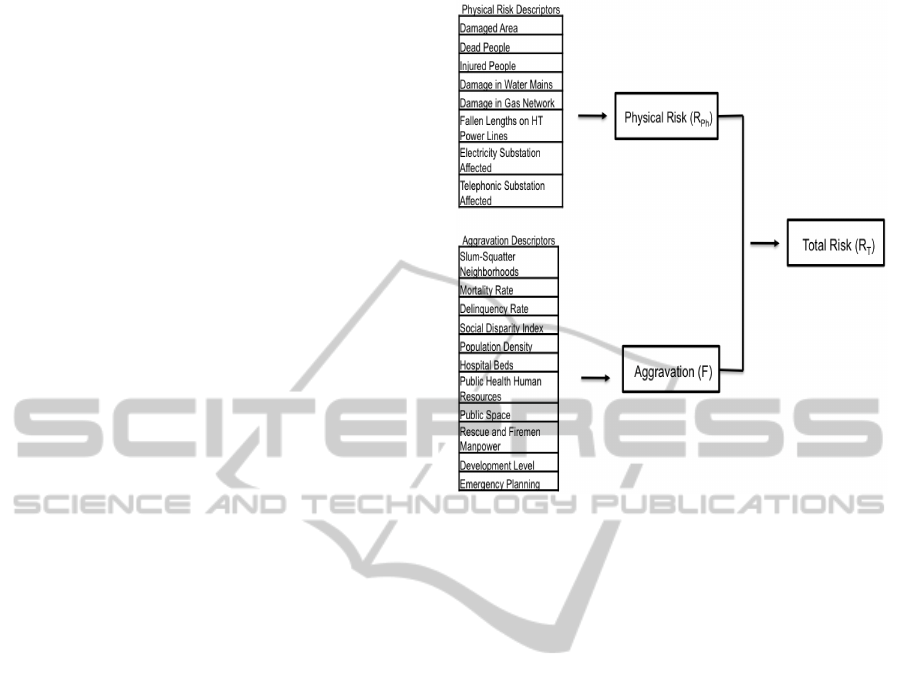
2 CARRE

NO’S MODEL

Taking as a base Cardona’s original model (2001),

Carre

no et al. (2012) proposed a seismic risk model

considering an integral (holistic) approach, regarding

seismic risk as a function of the potential damage on

assets (considering hazard intensities) plus the socioe-

conomic fragilities and lack of resilience of the con-

text. In this view, seismic risk would be the result

of physical risk, aggravated by social conditions and

lack of resilience capacities. Carre

no et al. model re-

lies in the use of descriptors for both: physical risk

(see the 8 physical risk descriptors of Figure 1) and

social aggravation (see the 11 aggravation descriptors

of Figure 1).

A conceptualization of Carre

no’s seismic risk

model can be seen in Figure 1.

Carre

no et al. (2012) obtained a seismic risk eval-

uation for Bogota city by means of indicators that

leads to the calculation of a total risk index. This is

obtained by direct application of Moncho’s equation

described in 1:

= R

(1 + F) (1)

where R

is the total risk, R

is the physical risk and

F is a aggravation coefﬁcient.

Figure 1: Carre

no et al. (2012) Holistic Seismic Risk

Model.

Thus, considering seismic risk as produced for

physical and an aggravation coefﬁcient; the risk in-

dex provides an approximate vision of the state of the

social capital infrastructure.

The physical risk is evaluated by using the Equa-

tion 2,

∑

i=1

(2)

where F

are the physical risk descriptors, w

are

their weights assessed by an analytic hierarchy pro-

cess (Carre

no et al., 2007; Saaty and Vargas, 1991),

and p the total number of considered descriptors in

the estimation. The physical risk descriptors values

can be obtained from previous physical risk evalua-

tions (damage scenarios) already made at the studied

location.

The aggravation coefﬁcient, F, depends on a

weighted sum of an aggravation descriptors set as-

sociated to socioeconomic fragility of the commu-

nity (F

SFi

) and lack of resilience of exposed context

LR j

), according to Equation 3,

F =

∑

i=1

SFi

∑

j=1

LR j

(3)

where w

SFi

and w

LR j

are the assessed weights on

each factors and m and n the total number of descrip-

tors for fragility and lack of resilience, respectively.

TacklingNon-linearityinSeismicRiskEstimationusingFuzzyMethods

533

The descriptors values were obtained from existent

databases and statistical data of the studied area.

The use of descriptors conforms an indirect tech-

nique to estimate a quantitative measure of change.

The ﬁnal aim is to describe intangible realities, hidden

trends or different classes of information in a com-

posite manner in order to present them all as quantiﬁ-

able entities that can be compared across space and

time scales. Basically, descriptors are an encapsu-

lation of a more complex reality using a single con-

struct, and they can be used solely as independent en-

tities of measure, or they can be aggregated to form

indices. Since an index is intended to describe a par-

ticular attribute, the attribute will determine a sort of

causality structure between it and the descriptors that

can be either reﬂective (the attribute inﬂuences the de-

scriptors) or formative (the descriptors inﬂuence the

attribute). The main difference is based in the internal

correlation of the descriptors. In the case of Carre

no’s

indices, there is a strong formative causality struc-

ture and therefore, the attributes can be assumed to

be interdependent. Therefore, the ﬁnal outcome of

descriptor’s aggregation would estimate the attribute

considering only a linear inﬂuence between descrip-

tors. Even if this assumption may be valid in some

circumstances, the main objective of the index is lost

since in fact, there is no a real measure of conditional-

ity or causality between descriptors, since none of the

indicators can be diminished or ampliﬁed by another

indicator, and therefore there is no way to assess non-

linearities or feedbacks that do exist in real systems.

In the same way Moncho’s equation presents a

linear relation between its physical and aggravation

components. Since the main assumption behind Mon-

cho’s equation is to consider physical risk as the main

seismic risk ”driver”, a clear consequence of assum-

ing linearity would be that the ﬁnal estimation of the

total seismic risk will rely in the existence, ﬁrst, of a

signiﬁcative physical risk value. Therefore, if a region

presents large social aggravation values, but the val-

ues for physical risk are small or medium for the same

area, the ﬁnal risk estimation will be small. This as-

sumptions can lead to a underestimation in the ﬁnal

risk estimation that can be misleading. For exam-

ple, an area with an important aggravation or social

vulnerability, might be severely affected by an earth-

quake of less intensity and the effects could be even

bigger and more spread, creating a series of unwanted

consequences that cannot be estimated using a linear

relationship between seismic risk components.

3 FUZZY SEISMIC RISK MODEL

The integral frame that we followed was built in the

believe that seismic risk can be viewed as the convo-

lution of two principal components: the social aggra-

vation and physical risk, which in turn forms the total

seismic risk of an urban center. The Fuzzy Seismic

Risk Model (FSRM) is divided in three main mod-

ules or sections: Social Aggravation, Physical Risk,

and Total Risk. Each one of them is conformed by dif-

ferent submodules. The main objective is to be able

to estimate seismic risk for an urban center consid-

ering social and physical aspects trough fuzzy infer-

ence modeling, therefore, not assuming a linear inter-

dependency between seismic risk components.

3.1 Aggravation Coefﬁcient

We built an aggravation coefﬁcient by re-deﬁning

and grouping Carre

no’s descriptors into three differ-

ent Fuzzy Inference Systems (FIS) called: resilience,

fragility and aggravation. Each subsystem is deﬁned

by a set of rules involving all proper descriptors. A

conceptualization of the different steps followed to es-

timate the aggravation coefﬁcient can be seen in Fig-

ure 2. The descriptors involved in each subsystem are

presented in the left hand side of Figure 2. FIS 1,

corresponds to the Fragility model and has as input

variables the Marginal Slums (MS), the Social Dis-

parity Index (SDI) and the Population Density (PD).

The output of FIS 1 is the level of fragility. On the

other hand, FIS 2 corresponds to the Resilience model

which have as input variables the Human Health Re-

sources (HHR), the Emergency Operability (EO) and

the Development Level (DL). The output of FIS 2 is

the resilience level. Finally, the Aggravation model

(FIS 3) takes as inputs the fragility and resilience lev-

els that are the output of FIS 1 and 2, respectively,

and infers the aggravation coefﬁcient. All the fuzzy

inference systems proposed in this research are based

on the Mamdani approach (Mamdani and Assilian,

1975), since it is the one that better represents the

uncertainty associated to the inputs (antecedents) and

the outputs (consequents) and allows to describe the

expertise in an intuitive and human-like manner.

The original 11 aggravation descriptors, presented

in Figure 1, were reduced to six variables by consid-

ering a subjective method which is based in the as-

sumption that certain descriptors reﬂects similar at-

tributes in terms of aggravation formation. For exam-

ple, descriptors called: mortality rate and delinquency

rate, are linked since they reﬂect negative social con-

sequences produced by a social structure failure, i.e.

a lack of access to certain social advantages, such as

SIMULTECH2015-5thInternationalConferenceonSimulationandModelingMethodologies,Technologiesand

Applications

534

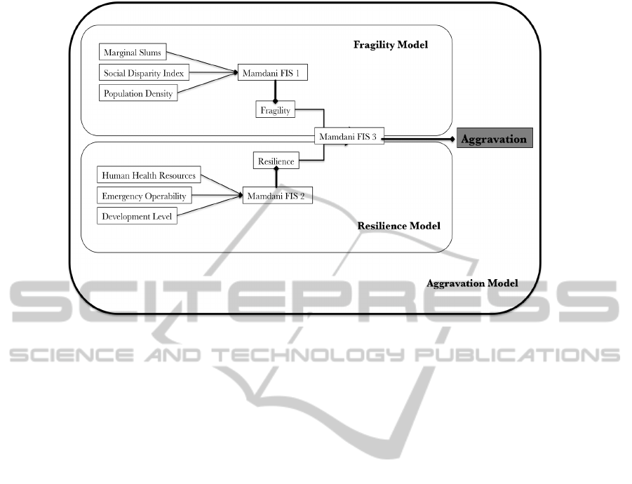
Figure 2: Mamdani fuzzy classical model structure to estimate Aggravation coefﬁcient.

an efﬁcient public health program, a strong marginal-

ization dynamics, no access to education or effec-

tive justice and law policies. Therefore, we consider

that these particular descriptors could be described us-

ing only the descriptor called social disparity index,

which is a fragility descriptor as well. In the case of

descriptors related to resilience we consider that de-

scriptors called: public space, hospital beds and emer-

gency personnel, are already reﬂected by the descrip-

tor named emergency operability, since the attributes

of the former descriptors are related with the capacity

of reaction when the emergency is being or has re-

cently occurred. Descriptors called: marginal slums,

population density, human health resources and de-

velopment level remain the same.

We used three linguistic labels deﬁned to qual-

ify each descriptor: low, medium and high, along

their respective universe of discourse. However, for

the FIS outputs, i.e. resilience, fragility and aggrava-

tion, we decided to use ﬁve labels: low, medium-low,

medium-high, high and very-high. We think that 3

classes is enough to accurately represent input vari-

ables of resilience and fragility models. Moreover, a

reduced number of classes implies a more compacted

and reduced set of fuzzy rules. To improve model’s

sensibility, we design membership functions in order

to consider the data variability. With these member-

ship functions we build a set of fuzzy rules that could

infer the behavior of the aggravation coefﬁcient us-

ing the three Mamdani fuzzy inference systems men-

tioned before (see Figure 2).

The development of the fuzzy rule base consid-

ers all possible combinations of descriptors linguis-

tic labels, therefore a total of 27 rules (3 descriptors)

characterized by 3 linguistic labels each) where re-

spectively used for infer fragility and resilience val-

ues. We think that the completeness of the fuzzy par-

tition is of great importance in this application. These

rules were intended to follow risk management litera-

ture which suggests possible outcomes when three of

these elements interact to form resilience or fragility.

At the other hand, the aggravation model, that has as

inputs resilience and fragility inferred values, char-

acterized by 5 classes each, is then composed of 25

fuzzy rules. In Table 1, the rules that conform the re-

silience FIS model are presented as an example. The

use of classical fuzzy systems, with well established

fuzzy inference theory, allow to build a solid model,

easily understandable by experts which leads towards

a deepest discussion over social vulnerability descrip-

tion and casuals non linear interrelations.

3.2 Physical Risk Coefﬁcient

In the holistic model presented in Figure 1, 8 descrip-

tors are associated with physical risk formation. Nev-

ertheless, we consider important to include another

descriptor already used in previous studies (Cardona,

2001; Carre

no, 2006) called damage in main roads,

due to its signiﬁcance for the analysis of seismic risk.

We categorized these new collection of physical risk

descriptors into three different models called: Prop-

erty Damage, Life Lines Sources Damage and Net-

work Damage, each of those was later framed into a

TacklingNon-linearityinSeismicRiskEstimationusingFuzzyMethods

535

Table 1: Rules that compose the resilience FIS model, used

to estimate the level of resilience. HHR = Human Health

Resources; DL = Development Level; EO = Emergency Op-

erability; R = Resilience; VH = very-high; H = high; MH =

medium-high; ML = medium-low; L = low.

1. If (HHR is L) and (DL is L) and (EO is L) then (R is L)

2. If (HHR is M) and (DL is M) and (EO is M) then (R is ML)

3. If (HHR is H) and (DL is H) and (EO is H) then (R is VH)

4. If (HHR is M) and (DL is L) and (EO is L) then (R is L)

5. If (HHR is H) and (DL is H) and (EO is L) then (R is M)

6. If (HHR is L) and (DL is M) and (EO is L) then (R is ML)

7. If (HHR is M) and (DL is M) and (EO is L) then (R is MH)

8. If (HHR is H) and (DL is M) and (EO is L) then (R is H)

9. If (HHR is L) and (DL is H) and (EO is L) then (R is MH)

10. If (HHR is M) and (DL is H) and (EO is L) then (R is MH)

11. If (HHR is H) and (DL is H) and (EO is L) then (R is H)

12. If (HHR is L) and (DL is L) and (EO is M) then (R is ML)

13. If (HHR is M) and (DL is L) and (EO is M) then (R is MH)

14. If (HHR is H) and (DL is L) and (EO is M) then (R is H)

15. If (HHR is L) and (DL is M) and (EO is M) then (R is MH)

16. If (HHR is H) and (DL is M) and (EO is M) then (R is H)

17. If (HHR is L) and (DL is H) and (EO is M) then (R is MH)

18. If (HHR is M) and (DL is H) and (EO is M) then (R is H)

19. If (HHR is H) and (DL is H) and (EO is M) then (R is H)

20. If (HHR is L) and (DL is L) and (EO is H) then (R is MH)

21. If (HHR is M) and (DL is L) and (EO is H) then (R is H)

22. If (HHR is H) and (DL is L) and (EO is L) then (R is H)

23. If (HHR is L) and (DL is M) and (EO is H) then (R is H)

24. If (HHR is M) and (DL is M) and (EO is H) then (R is VH)

25. If (HHR is H) and (DL is M) and (EO is H) then ((R is VH)

26. If (HHR is L) and (DL is H) and (EO is H) then (R is H)

27. If (HHR is M) and (DL is H) and (EO is H) then (R is VH)

FIS structure. Each model contains as inputs three of

the original descriptors. The structure of the physical

risk model can be seen in Figure 3. FIS 1, corresponds

to the Property Damage model and have as input vari-

ables: Damage Area (DA), Dead People (DP) and In-

jured People (INJ). The output of FIS 1 corresponds

to the level of property damage. The FIS 2 represents

the Life Lines Sources Damage model and have as in-

put variables: Telephonic Substation Affected (TSA),

Electrical Substation Affected (ESBA), and Damage

in Water Mains (DWM). The output of FIS 2 is the

level of damage to life lines sources. The FIS 3 corre-

sponds to the Network Damage model and have as in-

put variables: Damage in Gas Network (DGN), Fallen

Length of Electrical Lines (FLEN) and Damage in

Mains Roads (DMR). The output of FIS 3 is the net-

work damage level. FIS 4 corresponds to the Physical

Risk model, which takes as inputs the outputs of all

previous models, i.e. FIS 1, FIS 2 and FIS 3, and then

infers the physical risk coefﬁcient.

We decided to characterize each input variable

(descriptor) into 3 labels: low, medium and high, and

into ﬁve labels: low, medium-low, medium-high, high

and very-high, each FIS output, i.e. property dam-

age, life lines sources damage and network damage.

Therefore, as before, 27 fuzzy rules were obtained for

FIS 1, FIS 2 and FIS 3, and 25 for FIS 4. We also

designed the membership functions in order to reach

current data variability.

The rules of the Mamdani physical risk model are

Table 2: Rules that compose the physical risk FIS model,

used to estimate the physical risk coefﬁcient. LLSD = Life

Lines Sources Damage; PD = Property Damage; ND = Net-

work Damage; PR = Physical Risk; VH = very-high; H =

high; MH= medium-high; ML = medium-low; L = low.

1. If (LLSD is L) and (ND is L) and (PD is L) then (PR is L)

2. If (LLSD is M) and (ND is M) and (PD is M) then (PR is MH)

3. If (LLSD is H) and (ND is H) and (PD is H) then (PR is VH)

4. If (LLSD is M) and (ND is M) and (PD is M) then (PR is ML)

5. If (LLSD is H) and (ND is L) and (PD is L) then (PR is MH)

6. If (LLSD is L) and (ND is M) and (PD is L) then (PR is ML)

7. If (LLSD is M) and (ND is M) and (PD is L) then (PR is MH)

8. If (LLSD is H) and (ND is M) and (PD is L) then (PR is H)

9. If (LLSD is L) and (ND is H) and (PD is L) then (PR is MH)

10.If (LLSD is M) and (ND is H) and (PD is L) then (PR is M)

11.If (LLSD is H) and (ND is H) and (PD is L) then (PR is H)

12.If (LLSD is L) and (ND is L) and (PD is M) then (PR is ML)

13.If (LLSD is M) and (ND is L) and (PD is M) then (PR is MH)

14.If (LLSD is H) and (ND is L) and (PD is M) then (PR is H)

15.If (LLSD is L) and (ND is M) and (PD is M) then (PR is MH)

16.If (LLSD is H) and (ND is M) and (PD is M) then (PR is H)

17.If (LLSD is L) and (ND is alto) and (PD is M) then (PR is MH)

18.If (LLSD is M) and (ND is H) and (PD is M) then (PR is H)

19.If (LLSD is H) and (ND is H) and (PD is M) then (PR is H)

20.If (DLLS is L) and (ND is L) and (PD is H) then (PR is MH)

21.If (DLLS is M) and (ND is L) and (PD is H) then (PR is H)

22.If (DLLS is H) and (ND is L) and (PD is H) then (PR is H)

23.If (DLLS is L) and (ND is M) and (PD is H) then (PR is H)

24.If (DLLS is M) and (ND is M) and (PD is H) then (PR is VH)

25.If (DLLS is H) and (ND is M) and (PD is H) then (PR is VH)

26.If (DLLS is L) and (ND is H) and (PD is H) then (PR is H)

27.If (DLLS is M) and (ND is H) and (PD is H) then (PR is VH)

presented in Table 2 as an example.

3.3 Total Risk Coefﬁcient

The FIS called Total Risk will perform the convolu-

tion of all the previous FIS already developed, em-

bedded in one main structure that have as inputs the

variables representing the inferred values of physical

risk and social aggravation. In this case, both, inputs

and outputs, are characterized by the 5 labels men-

tioned in the previous section, obtaining a Mamdani

model composed of a set of 25 fuzzy rules to be used

in the inference process. As previously, the member-

ship functions are designed to represent the data vari-

ability. The Total Risk model structure can be seen in

Figure 4.

4 RESULTS: CITY OF BOGOTA

Colombia’s Capital is divided since 1992 into 20 ad-

ministrative Localities. However in our study we took

into account only 19 on these because the locality

called Sumapaz corresponds basically to the rural area

of the city. For the social aggravation coefﬁcient esti-

mation on each district we used statistical and demo-

graphic data from 2001 (Carre

no et al., 2012).

In Figures 5 and 6 we can see the aggravation val-

ues obtained by the proposed fuzzy model and the

index method, respectively. The general aggravation

SIMULTECH2015-5thInternationalConferenceonSimulationandModelingMethodologies,Technologiesand

Applications

536

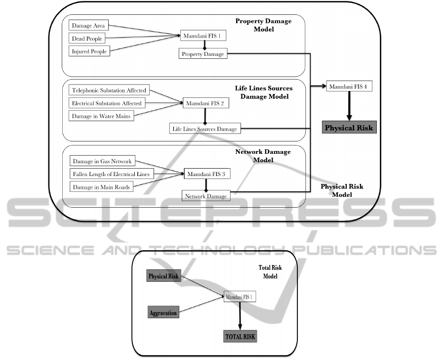
Figure 3: Conceptualization of Mamdani fuzzy classical model to estimate Physical Risk coefﬁcient.

Figure 4: Mamdani fuzzy classical model structure to estimate Total Risk coefﬁcient.

level seems to be lower for the FIS model when com-

pared with the index model. However, the FIS spatial

pattern distributes the highest values of aggravation

at the South-West part of the city as reported by in-

dex method, corresponding to the districts of: Ciudad

Bol

ıvar, Bosa, Usme, and San Cristobal. The East

part of the city remains with medium-low, while the

North-West part of the city presents medium-high ag-

gravation values. The index method reaches a very-

high value at South-West part of the city while the

northern part presents mostly a medium-low aggra-

vation value. In these ﬁgures we can see that even

there is no correct total match among the two meth-

ods, all of them preserve quite the same order in terms

of higher and lower aggravation values.

The physical risk coefﬁcient values are presented

in Figures 7 and 8 were the results of the fuzzy and

the index models are showed. Although the spatial

patterns changes, the highest values are encountered

in the north part of the city on both models, thus con-

taining the districts of: Usaquen, Suba Barrios Unidos

and Chapinero.

For the rest of the city, the fuzzy model esti-

mates homogeneous medium-high physical risk val-

ues, while in the index method map, this level of risk

is given only for the south part of the city.

The highest levels of physical risk are alike in the

two models. However, the change between higher and

lower physical risk values is more smooth in the fuzzy

model along 5 districts (Tunjuelito, Bosa, Ciudad

Kennedy, Fontib

on, Engativ

a and Antonio Nari

no),

when compared with the index model. Last, the to-

tal risk values were obtained for the 19 districts of

Bogot

a. Figures 9, 10 and 12 show the results for the

totally fuzzy, the Moncho’s-Index and the Moncho’s-

Fuzzy methods, respectively.

The proposed fuzzy model estimate a higher total

risk values for the city of Bogota and a more homoge-

neous spatial pattern. However, the areas with highest

levels, correspond also to those areas with the highest

TacklingNon-linearityinSeismicRiskEstimationusingFuzzyMethods

537

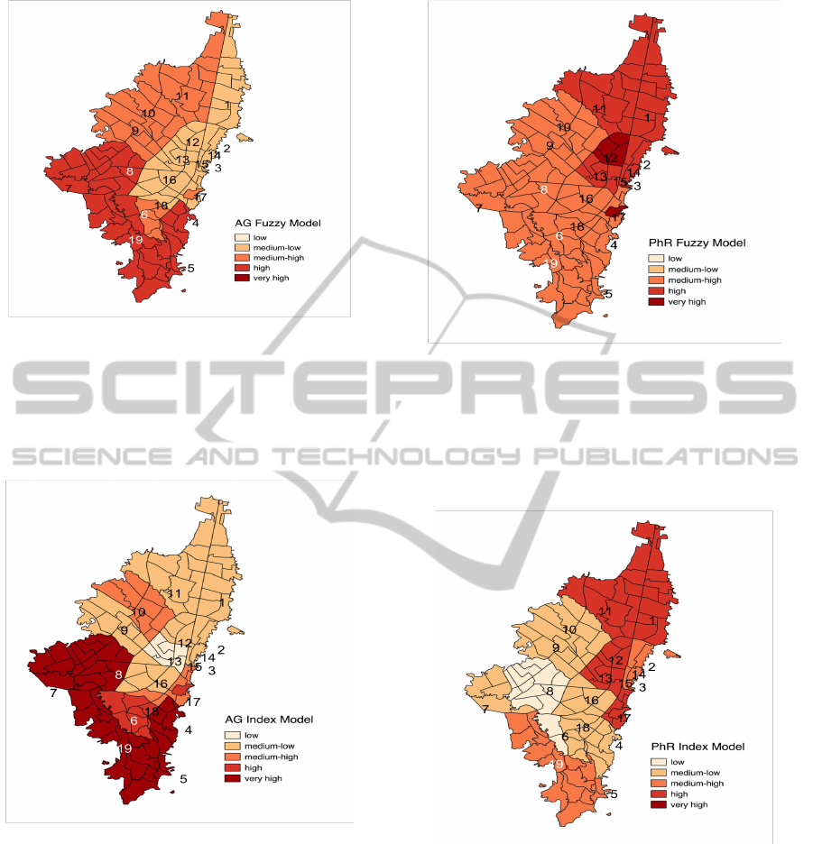
Figure 5: Aggravation coefﬁcients obtained by the proposed

Fuzzy Model: (1) Usaqu

en, (2) Chapinero, (3) Santa Fe,

(4) San Crist

obal, (5) Usme, (6) Tunjuelito, (7) Bosa, (8)

Ciudad Kennedy, (9) Fontib

on, (10) Engativ

a, (11) Suba,

(12) Barrios Unidos, (13) Teusaquillo, (14) M

artires, (15)

Antonio Nari

no, (16) Puente Aranda, (17) Candelaria, (18)

Rafael Uribe, (19) Ciudad Bol

ıvar.

Figure 6: Aggravation coefﬁcients obtained by the Index

Model:(1) Usaqu

en, (2) Chapinero, (3) Santa Fe, (4) San

Crist

obal, (5) Usme, (6) Tunjuelito, (7) Bosa, (8) Ciudad

Kennedy, (9) Fontib

on, (10) Engativ

a, (11) Suba, (12) Bar-

rios Unidos, (13) Teusaquillo, (14) M

artires, (15) Antonio

Nari

no, (16) Puente Aranda, (17) Candelaria, (18) Rafael

Uribe, (19) Ciudad Bol

ıvar.

levels according to the index method, even if the cur-

rent values are different. As the physical risk values

obtained by the fuzzy model are higher for a number

of Bogota localities, comparing with the same physi-

cal risk values obtained by the index method (see Fig-

ure 7 vs. Figure 8), the result is a more higher total

risk when using the fuzzy model (see Figure 9 vs. Fig-

Figure 7: Physical Risk coefﬁcients obtained by the pro-

posed Fuzzy Model: (1) Usaqu

en, (2) Chapinero, (3) Santa

Fe, (4) San Crist

obal, (5) Usme, (6) Tunjuelito, (7) Bosa, (8)

Ciudad Kennedy, (9) Fontib

on, (10) Engativ

a, (11) Suba,

(12) Barrios Unidos, (13) Teusaquillo, (14) M

artires, (15)

Antonio Nari

no, (16) Puente Aranda, (17) Candelaria, (18)

Rafael Uribe, (19) Ciudad Bol

ıvar.

Figure 8: Physical Risk coefﬁcients obtained by the Index

Model: (1) Usaqu

en, (2) Chapinero, (3) Santa Fe, (4) San

Crist

obal, (5) Usme, (6) Tunjuelito, (7) Bosa, (8) Ciudad

Kennedy, (9) Fontib

on, (10) Engativ

a, (11) Suba, (12) Bar-

rios Unidos, (13) Teusaquillo, (14) M

artires, (15) Antonio

Nari

no, (16) Puente Aranda, (17) Candelaria, (18) Rafael

Uribe, (19) Ciudad Bol

ıvar.

ure 10).

The total risk levels using the Moncho’s-Fuzzy

model (see Figure 12), show the highest level of seis-

mic risk at the northern part of the city, which is con-

gruent with the results from the other two models.

However, a direct application of Moncho’s equation

SIMULTECH2015-5thInternationalConferenceonSimulationandModelingMethodologies,Technologiesand

Applications

538

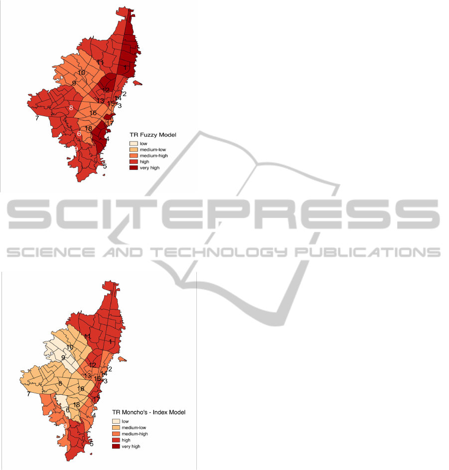
Figure 9: Total Risk coefﬁcients obtained by the proposed

Fuzzy models: (1) Usaqu

en, (2) Chapinero, (3) Santa Fe,

(4) San Crist

obal, (5) Usme, (6) Tunjuelito, (7) Bosa, (8)

Ciudad Kennedy, (9) Fontib

on, (10) Engativ

a, (11) Suba,

(12) Barrios Unidos, (13) Teusaquillo, (14) M

artires, (15)

Antonio Nari

no, (16) Puente Aranda, (17) Candelaria, (18)

Rafael Uribe, (19) Ciudad Bol

ıvar.

Figure 10: Total Risk coefﬁcients obtained by the Moncho’s

equation using aggravation and physical risk Index models

(Moncho’s-Index): (1) Usaqu

en, (2) Chapinero, (3) Santa

Fe, (4) San Crist

obal, (5) Usme, (6) Tunjuelito, (7) Bosa, (8)

Ciudad Kennedy, (9) Fontib

on, (10) Engativ

a, (11) Suba,

(12) Barrios Unidos, (13) Teusaquillo, (14) M

artires, (15)

Antonio Nari

no, (16) Puente Aranda, (17) Candelaria, (18)

Rafael Uribe, (19) Ciudad Bol

ıvar.

gives an homogeneous medium-high level for almost

all the city. As it can be seen, a direct application of

the Moncho’s equation vanishes the effect of social

aggravation to the total risk.

Figure 11 shows the total risk trend line over 19

districts of the city of Bogot

a. The variability esti-

mated by the fuzzy model resembles the one given

by the Moncho’s-Index model, especially at the right

hand side of the plot. However, the districts of: Santa

Fe, San Cristobal and Chapinero, show an opposite

trend from the values estimated by the index method.

The homogeneous values given by the Moncho’s-

Fuzzy model are more clearly seen in this graph,

although the highest risk values looks similar when

comparing with the others two alternative models.

According to the previous analysis, with the use

of classical fuzzy inference system methodology it is

plausible to achieve similar results to those obtained

from a more analytical method such as indexes, in

terms of district classiﬁcation, or in reproducing spa-

tial patterns of aggravation and physical risk. Fuzzy

logic inference capabilities can be exploited in a more

suitable way since the outputs from each FIS used in

the model are always fuzzy sets, giving the chance to

connect them trough a new FIS without loosing con-

sistency, allowing model completeness and avoiding

the assumption of interdependency between descrip-

tors, in order to calculate a ﬁnal risk output. There-

fore, one of the main advantages of the model is the

assumption of connectivity to create a risk value that

actually reﬂects the result of the correlation (both lin-

ear an non linear) between the components that were

assumed to inﬂuence seismic risk. It is interesting to

note how by not using Moncho’s equation for esti-

mate total risk allows to have a more clear vision of

the drivers of seismic risk in a non linear way. For

example, Figures 6, 8 and 10 shows the three com-

ponents of seismic risk estimated by index method.

Moncho’s equation follows the idea that there can be

only a high seismic risk if there is a high physical risk

value. If not, no matter if there is a large area pre-

senting a ”very high” aggravation value (the south-

eastern part of the city in ﬁgure 6), the ﬁnal index

will say that the total risk in that area is only be-

tween ”high and medium high”. The opposite behav-

ior is estimated by using fuzzy inferences (Figures

5, 7 and 9) where an area presenting high aggrava-

tions values, corresponds a proportional value of total

risk. As discussed, one of the steps needed to con-

form the designed FIS was in terms of the use of a

subjective methodology in order to reduce the orig-

inal dataset in order to avoid over correlation (dou-

ble counting) between variables. In more general risk

models, the number of variables involved, specially

in the social vulnerability part, can be in the order

of hundreds. Clearly a subjective scheme will not be

enough to reduce the number of variables and more

analytical methods are needed. The most common

way to reduce a data set relies in the use of statistical

TacklingNon-linearityinSeismicRiskEstimationusingFuzzyMethods

539

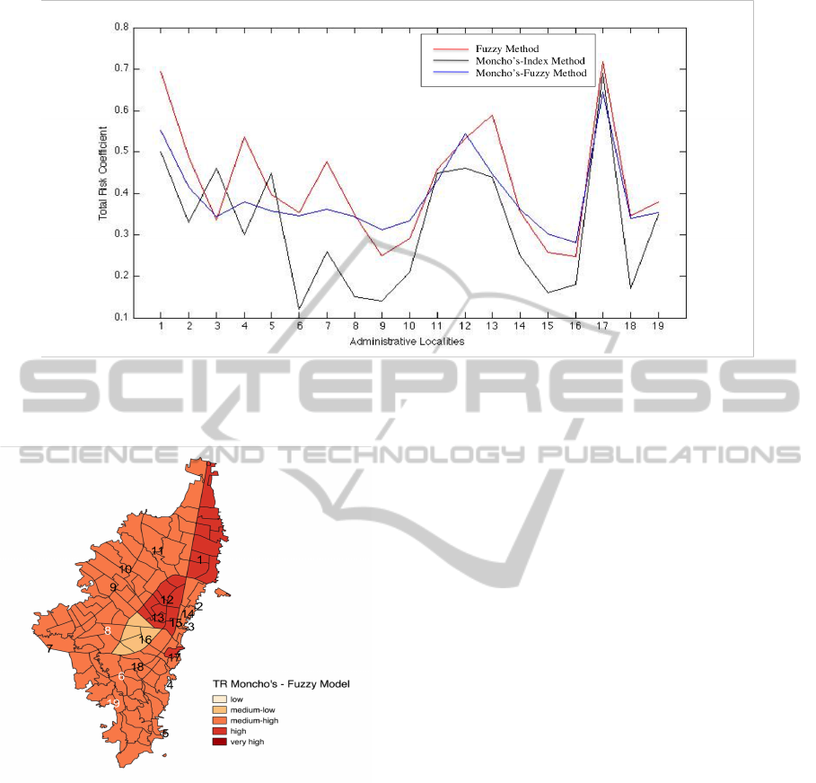
Figure 11: Total Risk coefﬁcients tendency: (1) Usaqu

en, (2) Chapinero, (3) Santa Fe, (4) San Crist

obal, (5) Usme, (6)

Tunjuelito, (7) Bosa, (8) Ciudad Kennedy, (9) Fontib

on, (10) Engativ

a, (11) Suba, (12) Barrios Unidos, (13) Teusaquillo, (14)

artires, (15) Antonio Nari

no, (16) Puente Aranda, (17) Candelaria, (18) Rafael Uribe, (19) Ciudad Bol

ıvar.

Figure 12: Total Risk coefﬁcients obtained by the Moncho’s

equation using aggravation and physical risk Fuzzy models

(Moncho’s-Fuzzy): (1) Usaqu

en, (2) Chapinero, (3) Santa

Fe, (4) San Crist

obal, (5) Usme, (6) Tunjuelito, (7) Bosa, (8)

Ciudad Kennedy, (9) Fontib

on, (10) Engativ

a, (11) Suba,

(12) Barrios Unidos, (13) Teusaquillo, (14) M

artires, (15)

Antonio Nari

no, (16) Puente Aranda, (17) Candelaria, (18)

Rafael Uribe, (19) Ciudad Bol

ıvar.

approaches such as linear correlation, principal com-

ponent analysis, or factor analysis. Nevertheless, all

of these methods assume as well, a linear correlation

between variables. At the same time, at the moment

of aggregate descriptors in order to build a composite

index, most of the time linear assumptions are used

which leads to lose information coming from the non

linear interdependency over descriptors that, in fact,

are the most importants. Therefore, the development

of tools to perform variable selection that do not fol-

low strictly linear assumptions are most needed.

5 CONCLUSIONS

We obtain a inference fuzzy model to make an estima-

tion of social aggravation over Bogota city using the

descriptors proposed in (Carre

no et al., 2012). Build-

ing inference compositional rules over the selected

descriptors, we were able to obtain a robust method

that resembles the identiﬁcation of relevant aspects

and characteristics of seismic risk of cities already

achieved by other consolidated method. The pro-

posed model displays simplicity, ﬂexibility and res-

olution capacities and does not assume linearity be-

tween the different components needed to obtain a ﬁ-

nal outcome.

REFERENCES

Cutter, S. L., Boruff, B. J., Shirley, W. L., (2003) Social

Vulnerability to Environmental Hazards. Social Sci-

ence Quarterly,84.

Cardona, O. D., (2001) Holistic evaluation of the seis-

mic risk using complex dynamic systems (in Span-

ish), PhD Thesis Technical University of Catalonia,

Barcelona, Spain.

Cardona, O.D., (2003) The need for rethinking the concepts

of Vulnerability and Risk from an Hollistic Perspec-

tive: a necessary review a criticism for effective Risk

SIMULTECH2015-5thInternationalConferenceonSimulationandModelingMethodologies,Technologiesand

Applications

540

Management, Mapping Vulnerability: Disasters, De-

veloping and People Chapter 3 Earthscan Publishers,

London.

Carre

no, M. L., Cardona, O. D., Barbat, A. H., (2007), Dis-

aster risk management performance index, Nat Haz-

ards 40 1-20.

Carre

no, M. L., Cardona, O.D., Barbat, A. H., (2012) New

methodology for urban seismic risk assessment from

a holistic perspective Bull Earthquake Eng, 10, 547-

565.

Mamdani, E. H., Assilian, S., (1975) An experiment in lin-

guistic synthesis with a fuzzy logic controller. Intern.

J. of Man-Machine Studies,7(1), 1-13.

Marulanda, M. C., Cardona, O. D., Barbat, A. H., (2009)

Robustness of the holistic seismic risk evaluation in

urban centers using the USRi, Nat Hazards, 49, 501-

516.

Kumpulainen, K., (2006) Vulnerability Concepts in Hazard

and Risk Assessment Geological Survey of Findand,

42, 65-74.

Saaty, T. L., Vargas, L. G., (1991) Prediction, projection,

and forecasting: applications of the analytical hier-

archy process in economics, ﬁnance, politics, games,

and sports, Kluwer Academic Publishers

TacklingNon-linearityinSeismicRiskEstimationusingFuzzyMethods

541