Inverse Kinematics of a Redundant Manipulator based on Conformal
Geometry using Geometric Approach
Je Seok Kim, Jin Han Jeong and Jahng Hyon Park
1
Department of Automotive Engineering, Hanyang University, Seoul, Korea
Keywords: Geometric Approach, Inverse Kinematics Analysis, Redundancy, Conformal Geometry, Joint Angles.
Abstract: This paper describes a geometrical approach for analysing the inverse kinematics of a 7 Degrees of Freedom
(DOF) redundant manipulator. The geometric approach is desirable since it provides complete and simple
solutions to the problem and determines the relationship between the joints and the end-effector without
iterative process. This paper introduces the approach to solve kinematic solution of 7 DOF in an intuitive way
using conformal geometric approach step by step. We finally present the comparison with pseudo inverse
solution which is the most well-known method in redundant manipulator kinematic problem at the same
simulation environment.
1 INTRODUCTION
A manipulators are designed to have the Degrees of
Freedom (DOF) only needed in the configuration
space, but have inherent problems, e.g., it is difficult
to avoid singularity or obstacles in the operating
space and lack of the adaptation to changes in
operating environments. Therefore, many studies are
conducted on a redundant manipulator in the form of
human arm with redundancy that uses remaining
DOF after performing given work to perform
additional work.
Generally, velocity kinematics algorithm and
geometric approach are used to analyse the inverse
kinematic of redundant manipulators. The velocity
kinematics algorithm (Whitney 1972, Liegeois 1977,
Baillieul 1985) is based on the generalized pseudo-
inverse to calculate the velocity transformation from
Cartesian to joint space. Pseudo-inverse of the
Jacobian matrix provides a possibility to solve for
approximate solutions. There is no exact velocity
solution for redundant robot. It increases the
possibility of singularity and causes cumulative errors
due to repeated integration of the value of speed. In
terms of the geometric approach, Tolani (Tolani,
Goswami et al. 2000) made a geometric approach by
the shape of 7-DOF manipulator into three joints of
shoulder, elbow, and wrist to express the movement
of human arm naturally in computer graphics, but it
was difficult to express the entities such as spheres
and circles in 3D spaces. This paper attempted to
reanalyse the study of Tolani in conformal geometry.
Conformal geometry is a mathematical language
that integrates various mathematical theories, such as
Projective Geometry, Quaternion, and Lie Algebra
for easy understanding and has been widely used
since the 1960s when Hestenes applied geometric
algebra to physics. Therefore, it is spotlighted as a
new method in robotics (Hildenbrand, Zamora et al.
2008, Aristidou and Lasenby 2011), computer vision
(Bayro-Corrochano, Reyes-Lozano et al. 2006,
Debaecker, Benosman et al. 2008, Ishida, Meguro et
al. 2013), and computer graphics (Wareham,
Cameron et al. 2005, Roa, Theoktisto et al. 2011).
Conformal geometry easily expresses intuitively and
mathematically the geometric entities, such as
spheres and circles, from geometric perspectives to
allow real-time calculations. For more details on
conformal geometry, refer to the paper by
Hildenbrand
(Hildenbrand 2012).
The inverse kinematics analysis of manipulators
in conformal geometry has already been conducted by
Hildenbrand (Hildenbrand, Lange et al. 2008)
and
Zamora (Zamora and Bayro-Corrochano 2004). They
used manipulators with 5- to 6-DOF only suitable for
given configuration space and the analysis was
possible only with simple geometric entities.
However, 7-DOF manipulator has redundancy and it
is necessary to optimize cost function.
Recently, many studies are conducted about cost
function in the inverse kinematics analysis of
179
Seok Kim J., Han Jeong J. and Hyon Park J..
Inverse Kinematics of a Redundant Manipulator based on Conformal Geometry using Geometric Approach.
DOI: 10.5220/0005535001790185
In Proceedings of the 12th International Conference on Informatics in Control, Automation and Robotics (ICINCO-2015), pages 179-185
ISBN: 978-989-758-122-9
Copyright
c
 2015 SCITEPRESS (Science and Technology Publications, Lda.)

redundant manipulators. Cost function was suggested
to make a movement similar to that of human arm
using redundant DOF and a method was suggested to
optimize cost function by choosing repetition and
manipulability(Kim, Miller et al. 2012). However,
most preceded studies have not considered the
dynamic properties of manipulators and can be weak
against vibration caused by link or outer load in the
actual behaviour of robots. This paper also studied a
method to determine the position of elbow by creating
and optimizing the cost function considering the
dynamic properties of manipulator for the inverse
kinematic analysis of redundant manipulator in
conformal geometry. Additionally, it created a
simulation to plan the target route for the manipulator
to accurately follow the indicated route, and
compared it with the velocity kinematics algorithm.
2 INVERSE KINEMATICS
In order to express the movement of end effector, the
kinematics must be analysed between the joint vector
and output vector. In this chapter, we present an
inverse kinematics which calculates each joint angles
from the configuration of the manipulator in
conformal geometry.
2.1 Redundant Manipulator
Figure 1 show a kinematic model of the redundant
manipulator in this paper. It consists of a series of
rigid links with seven joints (θ
1
, θ
2
, θ
3
, θ
4
, θ
5
, θ
6
, θ
7
).
In order to avoid complexity, we briefly set the basis
coordinate at the bottom.
Redundant manipulator
Before analysing the kinematics, the redundant
manipulator were analysed for simplicity. Since the
three axes adjacent to the base and three axes adjacent
to the end-effector meet at one point, we assume that
the kinematic model is as follows.
 The three joints (θ
1
, θ
2
, θ
3
) adjacent to the base
were assumed as the shoulder (3-DOF)
 The one joint (θ
4
) at the center of the
manipulator was assumed as the elbow (1-DOF)
The three joints (θ
5
, θ
6
, θ
7
) adjacent to the end-
effector were assumed as the wrist joint (3-DOF)
2.2 Redundant Degree of Freedom
For a position of the shoulder joint fixed to the base
and a position of the wrist joint along with a target
position and orientation of the end-effector, the
Figure 1: Redundant manipulator.
configuration of a redundant robot is fully defined if
and only if the position of the elbow joint is fully
specified.
As the position of shoulder is always on the z-axis
of global coordinates, it can be found from the point
expression of basic geometric entities in conformal
geometry. Eq. (1) expresses the position of shoulder,
P
2
.
2
213 1 0
1
2
de d e e

 P
(1)
As the position of wrist is determined by the given
target position and posture, it can be found using the
Rigid Body Motion of fixed object in conformal
geometry and is expressed by symbol,
6
P
.
The position of wrist,
6
P
, is defined as the point
which rotates the coordinates of target position,
t
P
,
by target posture (
,,
xyz
 ) and translates it by end-
effector,
4
d
, in the direction of –z axis, as shown in
Figure 2. To express the motion of fixed object,
Motor,
t
M
the geometric product of Rotor,
t
R
and
Translator,
t
T
is used as shown in Eq. (2):
123
43 43
exp exp exp
22 2
exp 1
22
y
x
z
t
t
ttt
eee
de de






  








 


R
T
M=RT
(2)
Point,
6
P
, is expressed as Eq. (3) by rigid body
motion of fixed object:
6 tt t
P=MPM

(3)
The position of elbow, P
4
, unlike the shoulder and
the wrist that are expressed by single points, is






ICINCO2015-12thInternationalConferenceonInformaticsinControl,AutomationandRobotics
180

expressed by infinite points and exists on the
consistent trajectory of a circle.
z

x

y

t
z
t
y
t
x
t
y
t
z
t
x
t
P
t
P
6
P
6
y
6
z
6
x
4
d
Figure 2: Wrist Point.
S
2
S
6
P
2
P
6
P
t
e
0
Z
4
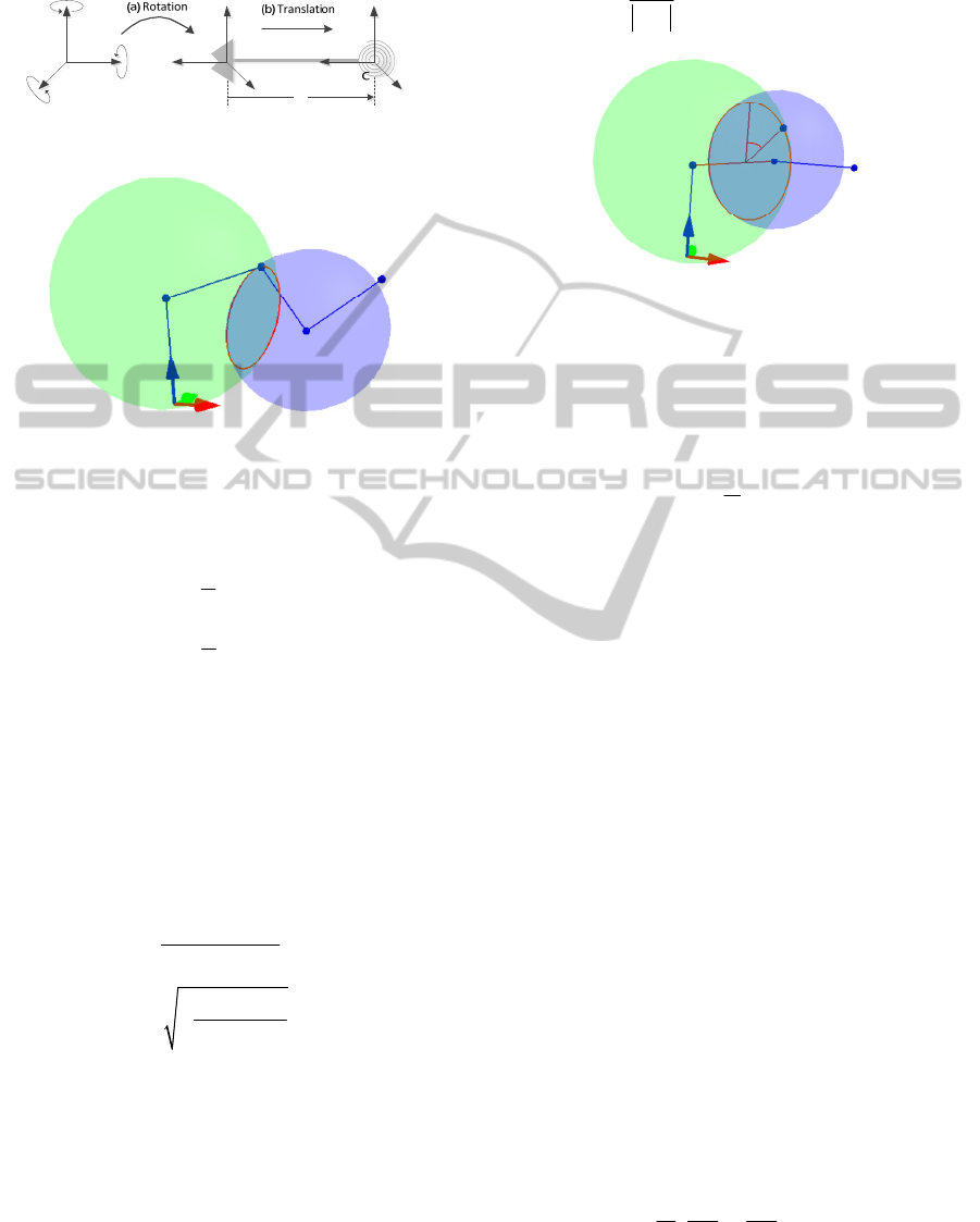
Figure 3: Intersection of spheres.
Let S
2
be a sphere with radius d
2
and center on
point P
2
, and S
6
be a sphere with radius d
3
and center
on point P
6
.
2
2
1
2
de


22
SP
(4)
2
3
1
2
de


66
SP
(5)
The intersection of sphere S
2
and S
6
is a circle Z
4
that represents all the possible locations of point P
4
known the positions of shoulder and wrist, as shown
in Figure 3.
426

Z=S S
(6)
Follows a study on (D'Orangeville and Lasenby
2003), the center P
c
and radius r
c
of the circle encoded
by the trivector (=circle) Z
4
is given by

44
44
c
e
ee




ZZ
P
ZZ
2
4
2
4
()
c
r
e



Z
Z
(7)
We have to define the redundancy angle ϕ to find
the point P
4
on the circle Z
4
. The position of the elbow
joint can be expressed as a function of ϕ (Tolani,
Goswami et al. 2000).
Let v be a normal vector of a plane containing the
origin e
0
, point P
2
, and point P
6
.

*
026 0 2 6
026
026
ee



π PP
π
v
π
(8)
e
0
P
2
P
t
P
4
φ
P
6
P
c
r
c
Figure 4: Elbow Circle.
A vector u perpendicular to the vector v is defined
as follows:
26 26
uRvR

(9)
where R
26
represents a rotor.
26 26
exp
4





RL
(10)
where L
26
is the rotation axis, represented by a
normalized bivector passing through the points P
2
and
P
6
.
Given the geometry depicted in Figure 4, the
position of the elbow can be expressed as follows:


4
() cos() sin()
cc
r

  PPu v
(11)
2.3 Minimization of Cost Function
This paper defined the cost function that minimizes
the force imposed on joints as operators operate the
manipulator considering the property that different
forces are imposed on manipulators according to the
location of elbow joint.
2.3.1 Euler-Lagrange Equation
Euler-Lagrange Equation is used to calculate the size
of force imposed on manipulator. As Euler-Lagrange
Equation uses generalized coordinates, it can be used
on any coordinates that express the position of objects
(Fowles and Cassiday 1999).
This paper defines generalized coordinates as the
position of elbow,
4
P
. Euler-Lagrange Equation is
defined as follows:
44
dL L
dt









F
PP

(12)
InverseKinematicsofaRedundantManipulatorbasedonConformalGeometryusingGeometricApproach
181

Lagrangian,
L
, is the difference between the kinetic
energy and the potential energy generated in the
center of mass of each link, as follows:
44
2
11
1
2
ii i i
ii
L
TU m mgz

 

r

(13
)
2.3.2 Center of Mass of Link
In the equation of Lagrangian,
L
, the center of mass
of each link was converted into the function of
position of elbow,
4
P
, with generalized coordinates.
First, the center of mass of each link was assumed as
consistent bars so it can always exist on the center of
link.
The center of mass of base link,
1
r
, is as follows
as it exists on the center of base link:
2
1
2

P
r
(14)
The center of mass of lower link,
2
r
, is the
geometric product of Translator,
2
T
, that transfers
from the position of shoulder,
2
P
, to the center of
mass of lower link, and can be simplified as follows:
42
2
42
22222
1
2
2
e





PP
T
PP
rTPTP

(15)
The center of mass of upper link,
3
r
, can be
simplified by the geometric product of Translator,
3
T
,
that transfers from position of wrist,
6
P
, to the center
of mass of lower link:
46
3
46
33636
1
2
2
e





PP
T
PP
rTPTP

(16)
The center of mass of lower link,
4
r
, is as shown
below as it exists in between the position of wrist,
6
P
,
and the target position,
t
P
:
6
46
2
t


PP
rP
(17)
2.3.3 Force on Elbow
When the simplified center of mass of each link is
applied to Eq. (13), Lagrangian,
L
, is as shown
below:



22
12 24
22
34 6 46
12 2 2 4
34 6 46
1
4
2
t
t
mm
L
mm
mz m z z
g
mz z mz z








 







 




PP
PP PP

 
(18
)
Therefore, the force applied onto the elbow joint
by Euler-Lagrange Equation is defined as follows:


4234336
1
2
4
mm ge m


 


FPP
 
(19)
2.3.4 Cost Function
The aforementioned size of force imposed on elbow
varies according to the position of elbow. Therefore,
the method of least squares (Haykin 1999) is used to
find the point,
4.i
P
, where the size of force imposed
on elbow joint on the circle,
4
Z
, becomes the
smallest. The cost function is defined as the function
about the size of force imposed on the elbow
according to the position of elbow joint. For this
purpose, Eq. (17) combines Sample Point,


4.ii

P
,
for the position of elbow and the size of force imposed
on the elbow joint,
4
F
, from Eq. (20), and expresses
the equation in a quartic polynomial to make it easier
to select the position of elbow. The following is
defined to express the results as similarly as possible,
and indicated by symbol,
E
:



01234
2
234
4012 3 4
1
,,,,
min
n
iiii
i
Ea a a a a
aa a a a








F
(20)
Here,
i

is the angle that rotates the base position
of elbow,
4.0
P
, by the rotation axis,
26
L
, and
4.i
F
is
the size of force imposed on the position of elbow,
4.i
P
, that is rotated by rotation angle,
i

.
Cost function,
E
, can be partially differentiated
by the factors of cost function,
0
a
,
1
a
,
2
a
,
3
a
, and
4
a
, as follows to find the angle,
i
x
, where cost function
is minimized:



234
4012 3 4
1
0
234
4012 3 4
1
1
4234
4012 3 4
1
4
2
2
2
n
iiii
i
n
iiiii
i
n
i iiii
i
E
aa a a a
a
E
aa a a a
a
E
aa a a a
a


 






     






     






     






F
F
F

(21
)
The equation equivalent to (23) is obtained by
equating to 0 the right hand side of (22). This matrix
form is known as Vandermonde matrix. The factor of
cost function can be calculated using this matrix:
ICINCO2015-12thInternationalConferenceonInformaticsinControl,AutomationandRobotics
182

1
4
4
11
1
0
25
1
4
1
11 1
45 8
4
4
4
1
11 1
nn
n
ii
ii
i
n
nn n
i
ii i
i
ii i
n
nn n
i
i
ii i
ii i
n
a
a
a


 

 




 

 




























 

 
F
F
F






(22)
The value that minimizes the cost function is the point
of inflection of quartic equation, so the value of this
point of inflection should be found. For this purpose,
the cost function of quartic equation is differentiated
and the value of differentiated cubic equation is
found. The value of cubic equation was found using
Cardano’s method (Wong and Sandler 1992). When
the minimum size of force is selected among the three
values, it becomes the position of value,
4
P
, that
becomes the smallest value.
2.4 Geometric Approach for Solving
the Joint Angles
As the positions of joints are decided, the joint angle
should be found. For the joint angle of manipulator,
the included angle created at the intersection of two
geometric entities (line, plane) can be calculated
using Eq. (23). For more details, refer to the paper by
(Hitzer 2013).
**
1
**
cos 








AB
AB
(23)
where A, B indicates the geometric entities and only
line and plane can be used as geometric entities.
However, since the range of usual principal value
of the function y=cos
-1
(x) is 0≤y≤π and the geometric
entities has orientation (Cameron and Lasenby 2008),
the solution for the joint angles cannot be simply
calculated using the Eq. (23). Therefore, given the
position of the elbow and wrist joint with respect to
the base frame, we propose the solution for inverse
kinematics that considers the orientation of the
geometric entities.
First, all of the auxiliary planes and lines that are
needed for the computation of the joint angles are
calculated. We need the following:
 The plane π
026
to which P
0
, P
2
and P
6
,

*
026 1 0 2 6
ee

π OPP
(24)
 The line L
24
though P
2
and P
6
,

*
24 2 2 4
e

LO PP
(25)
 The plane π
246
to which P
2
, P
4
and P
6
,
246 3 2 4 6
e

π OPPP
(26)
 The line L
46
though P
4
and P
6
,
46 4 4 6
e


LOPP
(27)
 The plane π
46t
to which P
4
, P
6
and P
t
,
46 5 4 6tt
e


π O PPP
(28)
 The line L
6t
though P
6
and P
t
,
666tt
e


LOPP
(29)
Now, we are able to compute solution for the first
six joint angles (i=1, 2,⋯ ,6)
1
113
exp
2
i
ii
e







RR
(30)
12 ii i
enR R

(31)
For O
i-2
, O
i
is the plane.
1
112
exp
2
i
ii
e







RR
(32)
31 ii i
enR R

(33)
For O
i-2
, O
i
is the line.


2
2
2
sgn acos
ii
iiii
ii










OO
OOn
OO
(34)
And the solution for last joint angle is
6
76 13
exp
2
e





RR
(35)
77127
enR R

(36)
7717
evR R

(37)
1 tt t
evR R

(38)


7
777
7
sgn acos
t
t
t







vv
vvn
vv
(39)
3 SIMULATION
3.1 Overview of Simulation
The overall program procedure for analyzing
proposed inverse kinematics algorithm of redundant
manipulators in conformal geometry is shown in
Figure 5.
We compared the performance of proposed
inverse kinematics analysis and velocity kinematics.
In this verification, we introduced a well-known
method with computational time and accuracy of the
solution.
InverseKinematicsofaRedundantManipulatorbasedonConformalGeometryusingGeometricApproach
183

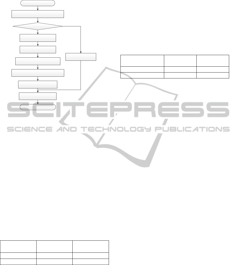
SetPos.andOri.ofGoal
GenerationPosition/SphereofShoulderand
Wrist
GenerationofElbowCircle
GenerationofElbowPos ition
GenerationofLink'sCenterofMass
Singularity?
CostFunctionusingEuler‐LagrangeEquation
MinimizationofCostFunction
GenerationofJointAngle
EndofInverseKinematics
NO
YES
SelectElbowPosition
Figure 5: Inverse kinematics algorithm of redundant
manipulators in conformal geometry.
3.2 Accuracy
The accuracy is the most essential evaluation points
in the inverse kinematic analysis since the accuracy
of the kinematic solution in a real time effects on the
control performance of the manipulation. In this
paper, we proved the inverse kinematic solutions by
comparing joint variables (position and orientation).
We created the multiple pose of the end effector
randomly and performed the test for the analysis
between the proposed method and the velocity
kinematics methods. We denoted the case that the
manipulate works inside the valid workspace in the
following table. In the case of velocity kinematics, it
has highly dependence of the initial joints variables
so that we set to zero.
Table 1: Comparison of accuracy.
Velocity
Kinematics
Proposed
method
Pos. error [m] 7.102E-8 6.834E-14
Ori. error [rad] 2.539E-7 1.117E-13
Finally, we get the competent solution both of
them. However, the velocity kinematic solution has
numerical singularity region depending on the initial
values.
3.3 Computation Time
The computational time plays an important role for
shortening control sample time. In the same way, we
tested the proposed kinematic solution with the
velocity kinematic solution at the 100 sample points
of the endpoint for the reasonable comparison. For the
experimental setup, we constructed the system with
3.6GHz CPU and 8GB RAM with LabVIEW and
performed 10 times iteratively.
Table 2: Comparison of computation time.
Velocity
Kinematics
Proposed
metho
d
Comp. time [sec] 7.320E-3 3.615E-3
Relative time 2.025 1
Table 2 represents the average time of the iterative
measurements for 10 times. The computational time
of the proposed method showed satisfactory
performance at average # μsec comparing to the
velocity kinematics. From the simulation results, we
concluded that the proposed kinematic method have
an advantage of real time analysis and get a unique
solution precisely at the same time.
4 CONCLUSIONS
For the operating a serial manipulator, the process of
solving inverse kinematics solution must be fast and
accurate at the same time since the solutions are used
to control the robot in a real time. Main contribution
of this research is that we applied conformal
geometric algebra to the redundant manipulator’s
kinematic solution which is intuitive and compact
geometric concept but fast and accurate.
In order to compare the kinematic solution, we
simulate at the same RTOS environment both pseudo
inverse method and proposed method with conformal
geometry. We finally concluded the kinematic
solution accuracy was more satisfactory compared to
previous methods and less computing time as well.
This made the robot maintain stability during the
motion for various operations.
ACKNOWLEDGEMENTS
This work was supported by the Research fund of the
Survivability Technology Defense Research Center
of the Agency for Defense Development of Korea
(No. UD120019OD).
ICINCO2015-12thInternationalConferenceonInformaticsinControl,AutomationandRobotics
184

REFERENCES
Aristidou, A. and J. Lasenby (2011). "FABRIK: A fast,
iterative solver for the Inverse Kinematics problem."
Graphical Models 73(5): 243-260.
Baillieul, J. (1985). Kinematic programming alternatives
for redundant manipulators. Robotics and Automation.
Proceedings. 1985 IEEE International Conference on,
IEEE.
Bayro-Corrochano, E., L. Reyes-Lozano and J. Zamora-
Esquivel (2006). "Conformal Geometric Algebra for
Robotic Vision."
Journal of Mathematical Imaging and
Vision 24
(1): 55-81.
Cameron, J. and J. Lasenby (2008). "Oriented conformal
geometric algebra." Advances in applied Clifford
algebras 18(3-4): 523-538.
D'Orangeville, C. and A. N. Lasenby (2003). Geometric
algebra for physicists,
Cambridge University Press.
Debaecker, T., R. Benosman and S.-H. Ieng (2008). Cone
of view camera model using conformal geometric
algebra for classic and panoramic image sensors. The
8th Workshop on Omnidirectional Vision, Camera
Networks and Non-classical Cameras-OMNIVIS,
Marseilles, France.
Fowles, G. R. and G. L. Cassiday (1999). Analytical
mechanics, Saunders college.
Haykin, S. (1999). "Adaptive filters." Signal Processing
Magazine 6.
Hildenbrand, D. (2012). Foundations of Geometric Algebra
Computing, Springer.
Hildenbrand, D., H. Lange, F. Stock and A. Koch (2008).
"Efficient inverse kinematics algorithm based on
conformal geometric algebra using reconfigurable
hardware.".
Hildenbrand, D., J. Zamora and E. Bayro-Corrochano
(2008). "Inverse Kinematics Computation in Computer
Graphics and Robotics Using Conformal Geometric
Algebra." Advances in Applied Clifford Algebras 18(3-
4): 699-713.
Hitzer, E. (2013). "Angles between subspaces." arXiv
preprint arXiv:1306.1629.
Ishida, H., J.-i. Meguro, Y. Kojima and T. Naito (2013).
"3D Road Boundary Detection Using Conformal
Geometric Algebra."
IPSJ Transactions on Computer
Vision and Applications 5
(0): 176-182.
Kim, H., L. M. Miller, N. Byl, G. Abrams and J. Rosen
(2012). "Redundancy resolution of the human arm and
an upper limb exoskeleton."
Biomedical Engineering,
IEEE Transactions on 59
(6): 1770-1779.
Liegeois, A. (1977). "Automatic Supervisory Control of the
Configuration and Behavior of Multibody
Mechanisms."
Systems, Man and Cybernetics, IEEE
Transactions on 7
(12): 868-871.
Roa, E., V. Theoktisto, M. Fairén and I. Navazo (2011).
GPU Collision Detection in Conformal Geometric
Space. V Ibero-American Symposium in Computer
Graphics SIACG.
Tolani, D., A. Goswami and N. I. Badler (2000). "Real-time
inverse kinematics techniques for anthropomorphic
limbs." Graphical models 62(5): 353-388.
Wareham, R., J. Cameron and J. Lasenby (2005).
Applications of conformal geometric algebra in
computer vision and graphics. Computer Algebra and
Geometric Algebra with Applications. Berlin
Heidelberg, Springer: 329-349.
Whitney, D. E. (1972). "The mathematics of coordinated
control of prosthetic arms and manipulators." Journal of
Dynamic Systems, Measurement, and Control 94(4):
303-309.
Wong, D. S. H. and S. I. Sandler (1992). "A theoretically
correct mixing rule for cubic equations of state." AIChE
Journal 38(5): 671-680.
Zamora, J. and E. Bayro-Corrochano (2004). Inverse
kinematics, fixation and grasping using conformal
geometric algebra. Intelligent Robots and Systems,
2004. (IROS 2004).
Proceedings. 2004 IEEE/RSJ
International Conference on
, IEEE.
InverseKinematicsofaRedundantManipulatorbasedonConformalGeometryusingGeometricApproach
185