Mobile Sensor Path Planning for Iceberg Monitoring

using a MILP Framework

Anders Albert and Lars Imsland

Department of Engineering Cybernetics, Norwegian University of Science and Technology, Trondheim, Norway

Keywords:

Optimization, Path Planning, UAV, UAS.

Abstract:

We look at the task of iceberg monitoring using a single mobile sensor, and we suggest a modular framework

for this. The focus is on path planning for which we come up with a novel strategy, which includes solving

a static optimization problem often to account for changes. We formulate the optimization problem in a

MILP framework, and we illustrate how this yields acceptable computational time for problem size of about

15 icebergs. We also suggest a tuning rule for weighting between different objectives in the optimization

formulation, which we demonstrate in simulations. Initializing the optimization with the previous solution

can improve computational time dramatically. Finally, we discuss how we easily can add extra features to our

framework.

1 INTRODUCTION

Unmanned Aerial Vehicles (UAVs), or more general

Unmannd Aerial Systems (UAS), have been studied

for a long time. The military has recognized the util-

ity of UAVs as early as WWI. During the Cold War

the efforts of developing UAVs for surveillance and

reconnaissance missions increased dramatically, and

the Vietnam War was the ﬁrst war where UAVs got put

into substantial use (Cook, 2007).

In modern times, UAVs performing surveillance and

reconnaissance missions see applications in civilian

life as well as the military. Examples of applications

are environmental monitoring - which include weather,

wildﬁre and polar monitoring (Chmaj and Selvaraj,

2015), trafﬁc surveillance (Peng et al., 2012), agricul-

ture (Watts et al., 2012) and much more.

In this paper we will study tracking of icebergs.

Radar, satellite imagery, shipboard sensors, drift buoys

and visual observation have traditionally been used for

the tracking and forecasting of icebergs (Timco et al.,

2005). However, we envision UAVs to be important in

the future of tracking icebergs (Eik, 2008). UAVs has

the advantage over satellites when comparing price

and maneuverability, in addition to spatial and tempo-

ral resolution. Satellites can only follow predeﬁned

trajectories. In the Northern hemisphere the satellite

coverage is pore, and you can expect only coverage

Research partly funded by Research Council of Norway,

RCN project no. 223254: CoE AMOS.

within hours interval. This calls for a real-time solu-

tion for monitoring icebergs, where we propose UAVs

as mobile sensors to be a cost-effective solution.

1.1 Contribution

Our contribution in this paper is a framework for mon-

itoring of moving targets with a single UAV. We in-

troduce a novel strategy for doing path planning. The

assumptions we make in Section 3 enable us to reduce

the path planning problem to the targets visitation prob-

lem (TVP) (Grundel and Jeffcoat, 2004). Furthermore,

we propose a formulation for this problem using Mixed

Integer Linear Programming in Section 3.1.

1.2 Previous Work

Path planning for UAVs is currently a popular research

topic, and it has been for the last 10 years. There are

many different approaches to path planning for UAVs

visiting different objects or targets. The most basic

approach to this problem is the Traveling Salesman

Problem (TSP). TSP is one of the most studied compu-

tational problems in the last 60 years(Applegate et al.,

2011) The TSP formulation for this problem is simply

to ﬁnd the shortest path that contains all targets. Refer-

ence (Applegate et al., 2011) may serve as a starting

point for TSP.

An extension of the TSP problem is to add proﬁts

to each target. TSP with proﬁts adds the objective of

collecting maximum of proﬁts without exceeding a

131

Albert A. and Imsland L..

Mobile Sensor Path Planning for Iceberg Monitoring using a MILP Framework.

DOI: 10.5220/0005521801310138

In Proceedings of the 12th International Conference on Informatics in Control, Automation and Robotics (ICINCO-2015), pages 131-138

ISBN: 978-989-758-122-9

 2015 SCITEPRESS (Science and Technology Publications, Lda.)

travel cost. A starting point for this research may be

(Feillet et al., 2005).

In this paper we use another approach with basis

in TSP, the targets visitation problem (TVP) (Grundel

and Jeffcoat, 2004). The difference between TVP and

TSP is that TVP also prioritize targets of high value

early in the visitation sequence. We will come back

to how we assign different values to the targets in our

case.

Besides formulations that take basis in TSP there

are multiple different approaches for a framework for

continuous trajectory planning. In (Haugen and Ims-

land, 2013), the path planning for mobile sensors is

formulated as a dynamic optimization problem. This

problem is discretized into a large-scale nonlinear pro-

gramming problem and solved. In another approach,

(Walton et al., 2014) formulate more complex dynam-

ics both for the mobile sensors and the targets. Then,

they present different complex problem formulations

and solve the optimization numerically.

In this paper we divide the path planning into dif-

ferent modules. In (Skoglar et al., 2012), they use a

similar approach and divide the sensor management

into different subtask. Then, they solve the path plan-

ning by using Bayesian estimation and search methods.

Another approach is to include all objectives into a sin-

gle objective function like (Pitre et al., 2009).

In (Alidaee et al., 2009), the authors formulate a

target search for

UAVs in a Mixed Integer Linear

Programming. This is similar to the formulation in

this paper.

This paper is organized as follows. We present the

problem formulation in Section 2. In Section 3, we

get into the task of path planning. First, we present the

strategy we apply to the path planning in this paper

with the appurtenant assumptions. Then, in Section 3.1

we formulate the optimization formulation and the con-

straints for the path planning. In Section 3.2 we come

up with a rule to assist tuning between the objectives

presented in Section 3.1. We handle the implementa-

tion and complexity of the path planning problem in

Section 4. We study a single case of monitoring 12

icebergs and show how weighting between the objec-

tives inﬂuences the solution in Section 5. Finally, we

discuss the result, conclude and discuss future work in

Section 6 and 7.

2 PROBLEM FORMULATION

In our case, icebergs are the desired target for moni-

toring and we use an UAV as the mobile sensor. Addi-

tionally, we have some a priori estimate of the location

of the icebergs to which we assign some uncertainty.

Ultimately, we desire an actuator input for the UAV,

which exploits our a priori information, iceberg and

UAV models, sensors, and possibly other information,

to keep track of the icebergs.

We choose to approach this problem in a modular

fashion. An advantage of dividing the problem into

different subtasks, is that it gets easier and safer to im-

plement. Two subtasks are, for example, path planning

and autopilot. If the path planning fails, the autopilot

will still keep the UAV in the air. The different tasks

can have different sampling time. While the UAV

will need to change its actuator input multiple times a

second, the path planning might not be necessary to

execute more than every other minute or even rarer.

Figure 1 illustrates the division and the dependen-

cies between the different subtasks. A more detailed

description of each task follows:

•

UAV: We view the UAV as a unit consisting of

both the physical structure of the airplane together

with an autopilot and measurement instruments.

We assume that the autopilot is able to set actuator

inputs for the plane based on waypoints. The UAV

must also have a sensors for discovering icebergs,

for instance thermal or optical cameras, and/or

radars.

•

Observer/Measurement Processor. The measure-

ments from the sensors must be processed. Fur-

thermore, a path planner will need a continuous

position estimate of all the icebergs.

•

Path Planner. A path planner will use the estimated

positions of icebergs to come up with a set of way-

points for the UAV that will minimize the position

uncertainty the icebergs. In addition, a path plan-

ner must manage the set of icebergs of interest. If

a new icebergs appear or icebergs leave the area

of interest, the path planner must update the set

of icebergs. Another task for the path planner is

to plan a path for searching for an icebergs not

located at the estimated position.

In this paper, we will not focus on using image pro-

cessing to obtain position and velocity measurements

of objects in water from a camera. An excellent refer-

ence for doing this is (Leira et al., 2015). The focus in

the paper will be the task of the path planning. We will

not go into the task of adding and removing icebergs

from the set of icebergs under observation, as this is

simple. Searching for icebergs that are not at their

estimated position might not be trivial, but it differs

from the path planning part and for that reason it will

not be considered here.

3 PATH PLANNING

The main task for the path planner in our framework

will be to take a set of iceberg position points and that

ICINCO2015-12thInternationalConferenceonInformaticsinControl,AutomationandRobotics

132

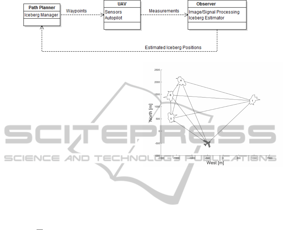
Figure 1: Framework for iceberg monitoring.

of the UAV and decide on a sequence for the UAV to

visit the icebergs.

Strategy

: We plan to solve the path planning prob-

lem often. Then, we apply only the ﬁrst iceberg of the

sequence to the UAV. When the UAV reach the iceberg,

we solve the path planning problem again and apply

the ﬁrst iceberg of the new sequence to the UAV, and

so on.

This strategy is inspired by model predictive con-

troll (MPC). MPC exploits knowledge of a process

model and constraints, and minimize some optimiza-

tion criteria to calculate a sequence of actuator inputs

over a control horizon. Then, MPC applies only the

ﬁrst actuator input of the sequence before repeating

the calculations using updated information about the

process. The controller continues to only apply the

ﬁrst actuator input of each solution sequence before

redoing the calculations.

To be able to apply this strategy, we need a fast and

efﬁcient path planning algorithm. The strategy also

enables us to make some assumptions and simpliﬁca-

tions:

•

We assume

UAV dynamics in the path plan-

ning, and merely decides the order of which the

UAV should visit the icebergs. This enables us

to simplify the formulation for the path planning

problem. This is a natural assumption if the ﬁeld

of view (FOV) of the UAV is larger than its turning

radius. If two or more icebergs are close, we can

consider them one point if the FOV will be able to

cover them both.

•

We assume that we have an initial estimate of the

position of the set of icebergs, for example from

satellite imagery. In addition, we assume that we

have an initial value for the position uncertainty of

each iceberg. We can calculate an uncertainty of

the position estimate based on the time since the

observation.

•

The icebergs move much slower than the UAV.

This enables us to consider the iceberg stationary

when formulating the path planning problem. A

typical iceberg velocity is of order 0.1 m/s (Eik,

2009), while we expect an UAV to move 22-25 m/s

(UAV Factory, 2012).

Figure 2 illustrates the problem. In the ﬁgure we

Figure 2: Path Planning Problem with UAV and 4 icebergs.

The numbers inside the icebergs are the position uncertainty

value for each iceberg.

have drawn the problem as a graph to make the simi-

larities to the traveling salesman problem (TSP) clear.

The UAV and each iceberg is a node in the graph. If

we do not consider the uncertainty of each iceberg and

with the stated assumptions we want a shortest path

that starts from the UAV and connects all the icebergs.

This is the traveling salesman problem.

The traveling salesman problem is a speciﬁc prob-

lem of the general class Mixed Integer Linear Pro-

gramming (MILP) (Bektas, 2006). MILP problems

are optimization problems containing integer variables

either in the objective function, in the constraints or in

both.

This motivates us to solve the path planning prob-

lem with an optimization approach. The ﬁrst objective

of the optimization approach will be, as with a TSP

problem, to ﬁnd the shortest distance between each

node in the graph. Second, we desire to reduce the

position uncertainty of each iceberg. We expect the

position uncertainty of each iceberg to vary with the

time since the UAV observed it. This objective reduces

to sort the iceberg according to their position uncer-

tainty. The optimization must weigh between these

two objectives.

An advantage with the strategy we choose is that

we do not need an accurate model of the icebergs.

Modeling icebergs is difﬁcult, especially since getting

other measurements than position and velocity from

MobileSensorPathPlanningforIcebergMonitoringusingaMILPFramework

133

the air is hard. By having a problem that we solve

often we can take new measurements into account

and thus compensate for model inaccuracies that will

accumulate over time.

3.1 Optimization Formulation for Path

Planner

We use a similar approach as (Bektas, 2006) to formu-

late the optimization problem in a MILP framework.

We consider

nodes in the optimization problem,

which is the number of icebergs in addition to the UAV.

Furthermore, we have two sets of optimization vari-

ables. The ﬁrst is a binary matrix,

path

, of dimension

N × N

. Each element,

path

(i, j)

, represent the path

from node

. The element is

if the path included

and

if not. The second optimization variable is an in-

teger vector,

, of length

. This contains the sequence

of each node in the visiting order.

We can now formulate the optimization problem as

min F(y

path

,t(i)) = −

∑

i=1

nodes

(i)(N −t(i))+ µD

(1)

The position uncertainty of each iceberg is represented

by a number in the vector

nodes

, where the ﬁrst ele-

ment is the position uncertainty of the UAV, which is 0.

A higher number represent a higher uncertainty, and

thus an increased desire to visit the iceberg.

is the

total distance traveled by the UAV and

is a tuning

variable we use to weight between the two objectives.

The total distance of the traveled path is

D =

∑

path

(i, j)d(i, j). (2)

The matrix

contains the distances from node

in element

d(i, j)

. Notice that this enables us to

include weather effects like wind by having a longer

distance to a point than from depending on ﬂying with

or against the wind.

Second, we must make sure that each node is not

visited and left more than once

∑

path

(i, j) ≤ 1 ∀ j and (3)

∑

path

(i, j) ≤ 1 ∀i. (4)

If we desire a circular path, these constraints should be

equality constraints. A linear path containing

nodes

needs N − 1 paths

N − 1 =

∑

i=1

∑

j=1

path

(i, j). (5)

The UAV must be the ﬁrst point in the path. To ensure

this we must set the ﬁrst element of the

vector equal

to 1:

t(1) = 1. (6)

We do not allow the UAV to visit an iceberg more

than once. To ensure this each element of the t vector

must be unique:

6= t

∀i 6= j. (7)

The values of

must be be within the number of

nodes in the problem:

1 ≤ t ≤ N. (8)

Finally, it is important that the optimal path is con-

nected. If we demand that each consecutive node that

are connected through a path is later in the visiting

sequence we avoid subcycles. The visiting sequence

is controlled by the t vector, making the constraint:

−t

i+1

≥ −N(1 − y

path

(i, j)) ∀i 6= j. (9)

3.2 Tuning

In the optimization formulation

weights between the

shortest distance and reducing the position uncertainty.

If the constant is set too high, the solution will be equal

to the TSP solution. Opposite, if the constant is set

too low the solution will be equal to a sorting of the

icebergs with the highest uncertainty ﬁrst. It is difﬁcult

to avoid having to tune this trade-off. However, it is

possible to deduce a tuning rule to help select the value

of the tuning constant.

The traveling distance for the UAV and the uncer-

tainty value are of different magnitude. To compare

them we need to scale them accordingly. First, we

suggest to calculate the maximum obtainable uncer-

tainty value. We can calculate this value by sorting the

uncertainty values of the iceberg in ascending order,

multiply element wise with a vector from 0 to

N − 1

and sum the vector:

1,max

N−1

∑

i=0

nodes,sorted

(i) · i (10)

Second, the matrix,

d(i, j)

, contains all the distances

from node

. We can calculate the average distance

for the entries in this matrix through the following

equation:

avg

∑

i=1

∑

j=1

d(i, j)

N(N − 1)

(11)

Finally, we calculate a rough estimate of the distance

traveled by multiply the average distance in the dis-

tance matrix by the number of paths we need in our

optimization problem:

est

= d

avg

(N − 1) (12)

ICINCO2015-12thInternationalConferenceonInformaticsinControl,AutomationandRobotics

134

Now, the objective function, equation

(1)

, using these

calculated constants is

F = −F

1,max

+ µD

est

(13)

We want to have the two terms in the objective to be

of comparable size, and a natural choice for

will

therefore be

µ =

1,max

est

. At this point we introduce an

additional tuning constant τ making the choice for µ:

µ = τ

1,max

est

(14)

This new tuning constant will be more intuitive to set.

A value of zero for

puts all the weight on minimizing

the position uncertainty of the iceberg, while a value

of one gives approximately equal weight to the two

objectives. However, as

is set to a large value (higher

than one), the weight is put on minimizing the traveling

distance of the UAV. In the simulations in Section 5

we will compare using different values for τ.

4 IMPLEMENTATION AND

COMPLEXITY OF PATH

PLANNING

MILP is in general an NP-complete problem with com-

puting time growing exponentially with problem size

(Mahajan and Ralphs, 2010). Therefore, since our

problem is a MILP problem, we will get an exponen-

tial growth in computational time with problem size.

However, with a modern computer and state-of-the-art

solver we will have an acceptable solution time for a

problem size of sufﬁciently small size.

To demonstrate the solution time of our problem

we solve the target visitation problem from equation

(1)

with an increasing problem size. To implement

the optimization formulation, we used the YALMIP

language developed by (Lofberg, 2004). To solve the

problem we use the solver CPLEX from IBM (IBM,

2011).

To setup up the target visitation problem we chose

to randomly set positions of the icebergs within a given

area. In addition, we randomly assign position uncer-

tainty values between 1 and 10 for each iceberg. Table

1 contains the parameters for setting up the problem.

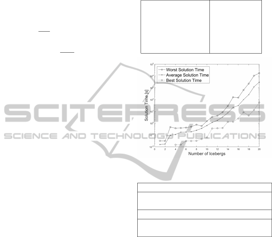
Figure 3 illustrate the worst case, average and best

solution time in seconds in a logarithmic plot. The

graph clearly illustrates the exponential rise in solution

time with the number of icebergs to track. However, if

the number of icebergs is kept at about 15 icebergs the

solution time is about 1-2 minutes. Table 2 lists some

of the solutions time in seconds.

There are two advantages with the strategy we have

chosen in regard to computational time. First, after

Table 1: Setup Parameters for each Problem of Different

Size.

Iceberg Area [5000m × 5000m]

Iceberg Uncertainty [1..10]

UAV position (-500m,-500m)

UAV Uncertainty 0

Number of Optimizations 50

τ 0.5

Figure 3: Computational time for different problem size.

Table 2: Average and Worst Case Computational Time.

Icebergs 2 6 10

Avg. sol. time [s] 0.02 0.18 0.64

Worst case sol. time [s] 0.03 0.42 1.50

Icebergs 12 16 20

Avg. sol. time [s] 1.71 31.20 2969.69

Worst case sol. time [s] 4.24 145.16 17269.17

solving the optimization problem one time we can use

the ﬁrst solution to initialize the next problem and so

on like an MPC. This is called a warm start can greatly

reduce the computational time. Second, if the solver

is not able to obtain a solution within a given time, the

UAV can use the next point in the previous solution

as the next waypoint. For these reasons the algorithm

can in practice handle up to 20 icebergs.

5 SIMULATION

In this section, we simulate iceberg monitoring with

12 icebergs and a single UAV. To demonstrate the path

planning algorithm from Section 3.1 with different

choices for τ from Section 3.2.

Before we go into the simulation results we present

MobileSensorPathPlanningforIcebergMonitoringusingaMILPFramework

135

the model we use for the UAV, the icebergs and the

position uncertainty of the icebergs.

5.1 Iceberg and UAV Models

For the UAV we use a Dubins Vehicle (Dubins, 1957)

as model



˙x







U cos(ψ)

U sin(ψ)





, (15)

here

is the position,

is the velocity,

is the head-

ing of the vehicle and

is the actuator of the UAV.

In addition, the actuator input must be within certain

limits

u ∈ [u

min

max

]. (16)

The UAV needs an autopilot to steer it from waypoint

to waypoint. We use the line of sight (LOS) algorithm

for the UAV autopilot described in section 10.3 of

(Fossen, 2011). In addition, we added integral action

in the controller with anti-windup from (Caharija et al.,

2012).

We model the iceberg as moving point with a known

velocity and velocity uncertainty

= v

+ w

(t), (17)

here

is the position,

is the known velocity and

(t) ∼ (0,Q

)

is the uncertainty in the velocity, which

have Gaussian distribution with a mean of zero and

variance of

. The dimension of

and

(t)

The subscript

highlights that all of these values are

different for each iceberg. This renders the estimate

model for each iceberg to be

= v

, (18)

where

is the estimated position of the iceberg.

We need to model the position uncertainty of each

iceberg. First, we consider the error in position esti-

mate deﬁned as

= ξ

−

. We can then calculate:

= w

(t) (19)

A reasonable assumption is that the variance in both

direction in the plane will be equal for an iceberg. This

means we can set

= q

2×2

. If we then deﬁne the

uncertainty,

, as the covariance of the estimation

error,

= E[

ξ (t)

(t)] (20)

and follow the calculations from section 8.1.1. in (Dan,

2006) we get:

= q

t (21)

When the icebergs comes within the FOV of the UAV

we set the uncertainty to zero. Combining this with

derivative of equation (21) we get:

= q ξ

/∈ FOV (22)

= 0 ξ

∈ FOV. (23)

5.2 Simulation Results

We ran simulations with 12 icebergs and a single UAV

to do the monitoring. The UAV and the iceberg were

spread out over an area of about

[5000m × 4000m]

The parameters we used in the simulation are in table

3. Notice that the same value for variance were used

for all iceberg. In addition, we used the same values

for

(t)

in all simulations. This is done to be able to

compare the effect of only changing the value for

through the simulations. All simulation run for a time

span of T = 1000 seconds.

Table 3: Simulation Parameters.

UAV Icebergs

= [−500, 500]

m q = 2.5 · 10

−2

∈

[0.0,0.4]m/s

FOV = 600m × 600m ξ

∈ [5 · 10

,5 · 10

]

max,min

= ±

tan(5

)

U = 22m/s, g = 9.81m/s

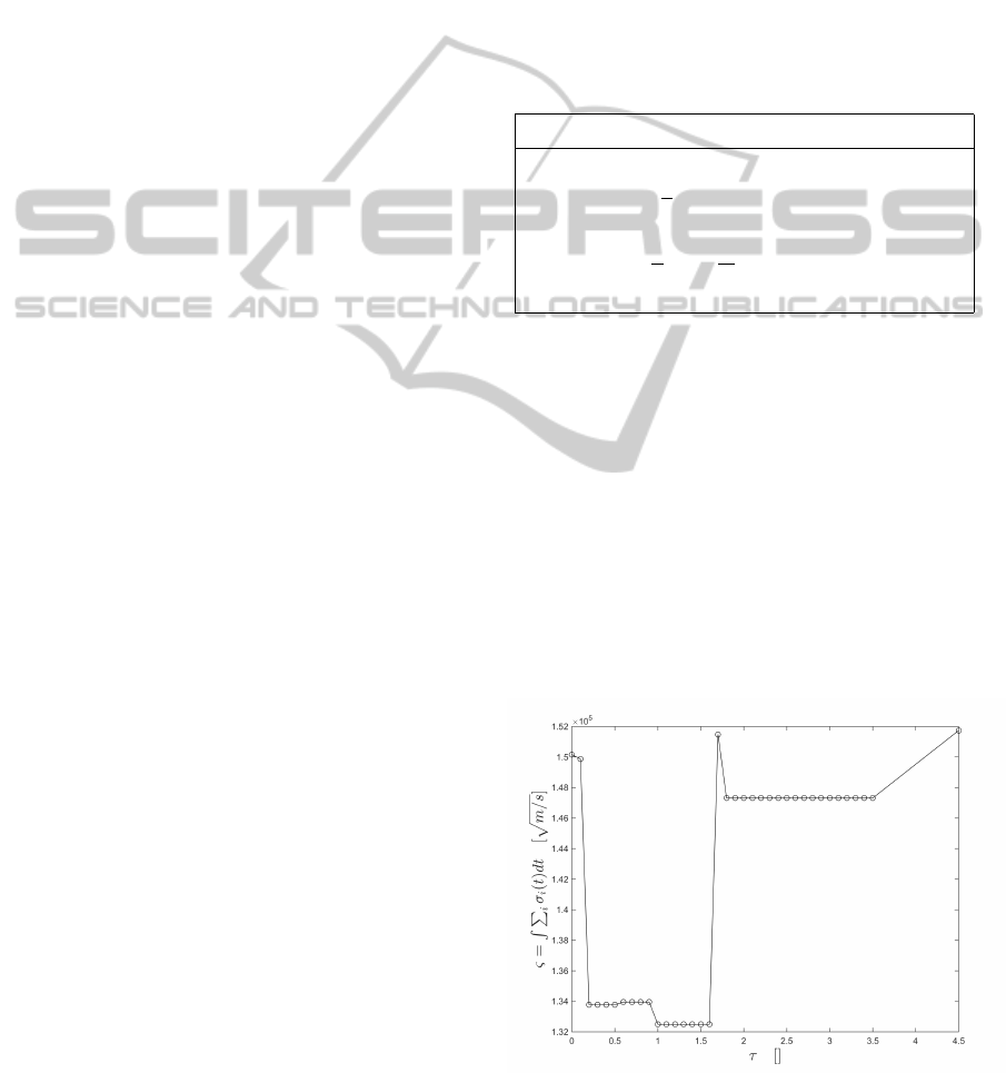
Our goal is to reduce the overall uncertainty of the

icebergs. To compare the simulations with the different

value of τ we calculate the performance metric:

ς =

N−1

∑

i=1

(t)dt (24)

The resulting integral of the total position uncer-

tainty is shown in Figure 4 as a function of

. With

the MPC-like implementation strategy presented in

this paper a high value for

will result in the UAV

being stuck in a loop between two points. The value

τ = 4.5

equals the TSP case, which is implemented

without the MPC-strategy.

Figure 4:

in relation to

for the case of monitoring 12

icebergs with a single UAV. The case of

= 4.5 is the TSP-

solution.

ICINCO2015-12thInternationalConferenceonInformaticsinControl,AutomationandRobotics

136

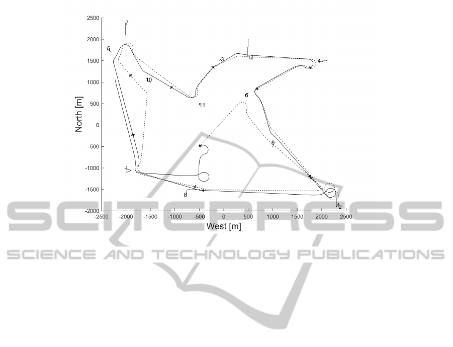
Figure 5: Simulation with 12 icebergs. The dotted path is the optimal path for this case with regard to the metric

. The whole

path is the TSP solution for this case.

Figure 5 shows two simulations of case with 12

icebergs. The UAV illustrated with the blue line is the

case

τ = 1.5

, which is optimal for this case. The other

case, where the UAV is plotted with a red line is the

TSP-solution for this case.

6 DISCUSSION

The strength of the framework we present in this article

is the simplicity. The objective function from equa-

tion

(1)

is intuitive and the tuning rule from Section

3.2 makes it easy to weight between the objectives.

Furthermore, the division of the objective of iceberg

monitoring into different task makes it easy to separate

between tasks like path planning and path following.

A challenge is to weight between the two objectives.

The optimal value for

will vary for each case. How-

ever, experience indicates that choosing

τ = 1

gives

a good trade-off between shortest path and highest

uncertainty ﬁrst.

Another strength of the division of task for the

framework is the ability to add extra features. A reason

for monitoring iceberg could be to protect an installa-

tion or ship. In such a case it will be more important to

prioritize icebergs that are close to the object you want

to protect. We can easily include this in our objective

function by assigning different values for the variance,

, for each iceberg based on the distance the iceberg

is from our object.

7 CONCLUSIONS AND FUTURE

WORK

In this paper we look at the monitoring of a set of

icebergs using a single UAV as a mobile sensor. Each

iceberg in the set has an estimated position with an

appurtenant position uncertainty. We suggest a frame-

work for dividing the task into different subtask sepa-

rating path planning, autopilot and observer, and we

focus on the path planning. For the path planning we

come up with a strategy consisting of solving an opti-

mization problem with the icebergs as stationary. The

result of the optimization yields a sequence for visiting

the icebergs. We apply only the ﬁrst iceberg in the op-

timal sequence. When the UAV discovers that iceberg,

we solve the optimization again. The advantage of

solving the optimization this way is fast computational

time and at the same time account for model inaccu-

racies and changes over time by solving the problem

often. In the optimization we use both the objective

of achieving shortest distance and visiting the iceberg

with highest position uncertainty ﬁrst. To implement

the optimization formulation we use a MILP frame-

work. We also suggest a rule to help tuning between

the two objectives in the optimization formulation us-

ing a single parameter

. In simulation we demonstrate

how different choices of

inﬂuences the solution for

a single case. We use experience with different cases

to come with a recommendation for a value of

. The

complexity of our problem is NP-complete. However,

with the number of icebergs at about 15, the compu-

MobileSensorPathPlanningforIcebergMonitoringusingaMILPFramework

137

tational time of our problem is acceptable. Also by

initializing our problem with the previous solution, we

can yield acceptable computational time for about 20

icebergs. Finally, we discuss how our framework eas-

ily can be extended. For example different weighting

between icebergs based on their location and not only

the time since their last observation.

Future work include:

•

Extend the path planning to include management

and recovery of lost icebergs.

•

Perform experiments with UAV for proof of con-

cept

• Extend the algorithm to allow multiple UAVs

REFERENCES

Alidaee, B., Wang, H. B., and Landram, F. (2009). A

note on integer programming formulations of the real-

time optimal scheduling and ﬂight path selection of

uavs. Ieee Transactions on Control Systems Technol-

ogy, 17(4):839–843.

Applegate, D. L., Bixby, R. E., Chvatal, V., and Cook, W. J.

(2011). The Traveling Salesman Problem: a Compu-

tational Study. Princeton University Press, Princeton,

1st edition.

Bektas, T. (2006). The multiple traveling salesman problem:

an overview of formulations and solution procedures.

Omega-International Journal of Management Science,

34(3):209–219.

Caharija, W., Candeloro, M., Pettersen, K. Y., and Srensen,

A. J. (2012). Relative velocity control and integral los

for path following of underactuated surface vessels. In

Proc. of the 9th IFAC Conference on Manoeuvring and

Control of Marine Craft.

Chmaj, G. and Selvaraj, H. (2015). Distributed processing

applications for uav/drones: A survey. In Advances

in Intelligent Systems and Computing, volume 1089,

pages 449–454.

Cook, K. L. B. (2007). The silent force multiplier: The

history and role of uavs in warfare. In IEEE Aerospace

Conference, 3 - 7 March, 2007. Inst. of Elec. and Elec.

Eng. Computer Society.

Dan, S. (2006). Optimal state estimation Kalman H and

nonlinear approaches. New York: Wiley Interscience

Publication, 1st edition.

Dubins, L. E. (1957). On curves of minimal length with a

constraint on average curvature, and with prescribed

initial and terminal positions and tangents. American

Journal of mathematics, pages 497–516.

Eik, K. (2008). Review of experiences within ice and iceberg

management. Journal of Navigation, 61(04):557–572.

Eik, K. (2009). Iceberg drift modelling and validation of

applied metocean hindcast data. Cold Regions Science

and Technology, 57(2-3):67–90.

Feillet, D., Dejax, P., and Gendreau, M. (2005). Travel-

ing salesman problems with proﬁts. Transportation

Science, 39(2):188–205.

Fossen, T. I. (2011). Handbook of marine craft hydrody-

namics and motion control. John Wiley & Sons, 1st

edition.

Grundel, D. A. and Jeffcoat, D. E. (2004). Formulation and

solution of the target visitation problem. In Collec-

tion of Technical Papers - AIAA 1st Intelligent Systems

Technical Conference, 20 - 23 September 20, 2004, vol-

ume 1, pages 1–6. American Institute of Aeronautics

and Astronautics Inc.

Haugen, J. and Imsland, L. (2013). Optimization-based

autonomous remote sensing of surface objects using

an unmanned aerial vehicle. In 12th European Control

Conference, ECC 2013, 17 - 19 July 17, 2013, pages

1242–1249. IEEE Computer Society.

IBM (2011). Ibm ilog cplex optimization studio cplex users

manual. URL: http://www.ibm.com.

Leira, F. S., Johansen, T. A., and Fossen, T. I. (2015). Auto-

matic detection, classiﬁcation and tracking of objects

in the ocean surface from uavs using a thermal camera.

In IEEE Aerospace Conference, March 7-14. 2015.

Lofberg, J. (2004). Yalmip: A toolbox for modeling and

optimization in matlab. In Proceedings of the IEEE

International Symposium on Computer-Aided Control

System Design, pages 284–289.

Mahajan, A. and Ralphs, T. (2010). On the complexity of

selecting disjunctions in integer programming. SIAM

Journal on Optimization, 20(5):2181–2198.

Peng, Z. R., Liu, X. F., Zhang, L. Y., and Sun, J. (2012).

Research progress and prospect of uav applications in

transportation information collection. Jiaotong Yunshu

Gongcheng Xuebao/Journal of Trafﬁc and Transporta-

tion Engineering, 12(6):119–126.

Pitre, R. R., Li, X. R., and DelBalzo, D. (2009). A new

performance metric for search and track missions 2:

Design and application to uav search. In 12th Interna-

tional Conference on Information Fusion, FUSION 6 -

9 July, pages 1108–1114. IEEE Computer Society.

Skoglar, P., Orguner, U., Tornqvist, D., and Gustafsson, F.

(2012). Road target search and tracking with gimballed

vision sensor on an unmanned aerial vehicle. Remote

Sensing, 4(7):2076–2111.

Timco, G., Gorman, B., Falkingham, J., and O’Connell, B.

(2005). Scoping study: Ice information requirements

for marine transportation of natural gas from the high

arctic. Technical Report, prepared for: Climate Change

Technology and Innovation Initiative Unconventional

Gas Supply.

UAV Factory (2012). Penguin b datasheet. URL:

http://www.uavfactory.com.

Walton, C. L., Gong, Q., Kaminer, I., and Royset, J. O.

(2014). Optimal motion planning for searching for

uncertain targets. In 19th World Congress The Inter-

national Federation of Automatic Control, Cape Town,

South Africa. Agust 24-29, 2014.

Watts, A. C., Ambrosia, V. G., and Hinkley, E. A. (2012).

Unmanned aircraft systems in remote sensing and sci-

entiﬁc research: Classiﬁcation and considerations of

use. Remote Sensing, 4(6):1671–1692.

ICINCO2015-12thInternationalConferenceonInformaticsinControl,AutomationandRobotics

138