
Downscaling Daily Temperature with Evolutionary Artificial Neural
Networks
Min Shi
Norwegian Meteorological Institute, Oslo, Norway
Keywords: Temperature, Downscaling, Artificial Neural Networks, Evolutionary Algorithms.
Abstract: The spatial resolution of climate data generated by general circulation models (GCMs) is usually too coarse
to present regional or local features and dynamics. State of the art research with Artificial Neural Networks
(ANNs) for the downscaling of GCMs mainly uses back-propagation algorithm as a training approach. This
paper applies another training approach of ANNs, Evolutionary Algorithm. The combined algorithm names
neuroevolutionary (NE) algorithm. We investigate and evaluate the use of the NE algorithms in statistical
downscaling by generating temperature estimates at interior points given information from a lattice of
surrounding locations. The results of our experiments indicate that NE algorithms can be efficient
alternative downscaling methods for daily temperatures.
1 INTRODUCTION
General Circulation Models (GCMs) numerically
simulate the present climate as well as project future
climate. The output of GCMs, however, cannot be
applied to many impact studies due to their
relatively coarse spatial resolution (in the order of
from 200 km × 200 km to 300 km × 300 km).
Downscaling, as an emerge technique, is able to
model data from large-scale to smaller-scale.
Various downscaling techniques have been proposed
in literatures (Xu, 1999). In general, these
techniques can be divided into two major categories:
dynamic downscaling and statistical downscaling.
Dynamic downscaling works based on physically
regional climate models, which is computationally
expensive. Comparing with dynamic downscaling,
statistical downscaling is computationally less
demanding. The methods of statistical downscaling
are to build models to find the relationship between
large regional climatic variables, such as
temperature, precipitation, pressure etc., and sub-
regional climatic variables. The major sub-
categories of statistical downscaling techniques
include weather classification schemes, weather
generators and regression methods, in which
regression methods are most widely used.
Artificial Neural Networks (ANNs), as non-
linear regression models, have shown high potential
for complex, non-linear and time-varying input-
output mapping (Specht, 1991; Hecht-Nielsen, 1989;
Kohonen et al., 1988; Lu et al., 1998). There are
various successful applications of ANNs to
statistical downscaling in last decades. Snell et al.
(1999) introduced ANNs to the downscaling of
GCMs and evaluated their use to generate
temperature estimates at 11 locations given
information from a lattice of surrounding locations.
Their results indicated that ANNs can be used to
interpolate temperature data from a grid structure to
interior points with a high degree of accuracy.
Cawley et al. (2003) presented ANN models in
statistical downscaling of daily rainfall at stations
covering the north-west of the United Kingdom.
Their main purpose was to compare different error
metrics for training ANNs in statistical downscaling.
Dibike and Coulibaly (2006) investigated the
capacities temporal neural networks (TNNs) as
downscaling method of daily precipitation and
temperature series for a region in northern Quebec,
Canada. Their experiments demonstrated that the
TNN model mostly outperforms other statistic
models. Chadwick et al. (2011) developed an ANN
model to construct a relationship between a GCM
and corresponding nested RCM fields for
downscaling of GCM temperature and precipitation.
Their ANN model was able to reproduce the RCM
climate change signal very well, particularly for the
full European domain. Most of the previous
237
Shi M..
Downscaling Daily Temperature with Evolutionary Artificial Neural Networks.
DOI: 10.5220/0005507002370243
In Proceedings of the 5th International Conference on Simulation and Modeling Methodologies, Technologies and Applications (SIMULTECH-2015),
pages 237-243
ISBN: 978-989-758-120-5
Copyright
c
2015 SCITEPRESS (Science and Technology Publications, Lda.)
researches with ANNs employed classic back-
propagation (BP) as leaning approach to train ANNs
for the downscaling of GCMs. However, it has been
well-known that BP algorithms have difficulty with
local optima, slower convergence and longer
training times (Cuéllar et al., 2006).
In this research, we are going to explore and
evaluate GCM downscaling with ANNs by using
evolutionary algorithms, also names
neuroevolutionary algorithms. Evolutionary
techniques have been widely and successfully
applied to data models optimization (Eiben et al.,
1999; Buche et al., 2005; Regis and Shoemaker,
2004), but rarely introduced into statistical
downscaling. Genetic Programming (GP) is the
major evolutionary technique that has been
investigated in atmospheric downscaling, which has
been also demonstrated to be superior to the widely
used Statistical Down-Scaling Model (SDSM)
(Coulibaly, 2004; Zerenner et al., 2014).
This paper presents our initial results of a study
for large-scale spatial interpolation of daily
temperature at stations in south of Norway. The
performances of our model indicate good potential
of the neuroevolutionary technique as an effective
statistical downscaling method for maximum
temperature estimation. The rest of the paper is
organized as follows: Section 2 describes the
methodolology of our model. The experimental
results and discussion on the performance of our
model are presented in section 3. The concluding
remarks, including future work, are given in the last
section.
2 METHODS
2.1 Artificial Neural Networks
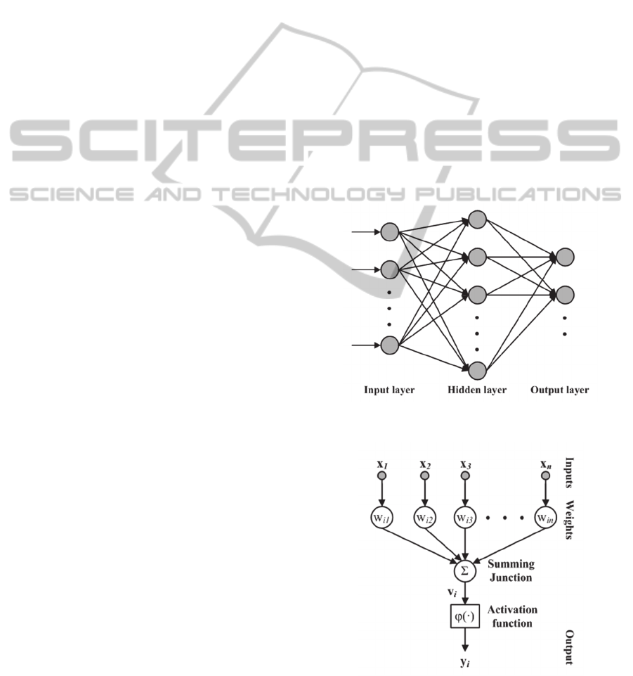
An artificial neural network (ANN) is a
mathematical model that simulates biological neural
networks, which can be used for performing tasks
such as classification, control, recognition,
prediction, regression and so on. It consists of a set
of interconnected nodes. Each node can be regarded
as a neuron and each connection between two nodes
can be regarded as a synapse. The mathematical
models of an ANN and a neuron are shown in Figure
1 and Figure 2. There are three basic elements in an
ANN: node, weight and activation function. A node
represents a neuron. The weights between
interconnected nodes of an ANN model the
synapses. Each weight is a real number, which
represents the strength of a connection. A positive
value reflects an excitatory connection, while a
negative weight reflects an inhibitory connection.
All of the inputs are multiplied by the weights and
summed according to the following expression:
n
j
jjii
xwv
1
,
where
njx
j
,1,
are the inputs to the node
i
, and
ji
w
,
is the weight of the connection between the
node
i
and the input
j
. The summing function is
input into an activation function. The output of the
node
i
y
will be the outcome of the activation
function on the value of
i
v
. The main purpose of
using the activation function is to control the
amplitude of the output of each node. Common
activation functions used in ANNs include step
function, piecewise-linear function, sigmoid
function and hyperbolic tangent function, in which
sigmoid function is mostly used, as well as applied
to our model.
Figure 1: The model of an ANN.
Figure 2: The model of a neuron.
SIMULTECH2015-5thInternationalConferenceonSimulationandModelingMethodologies,Technologiesand
Applications
238

After defining the weights, activation function
and topology of an ANN, we will be able to
calculate the output of the ANN for a particular
input vector. Usually, the output of an ANN has no
meaning before the ANN is trained, unless the ANN
is configured using prior knowledge. Training is a
process of adjusting the weights, topologies or
activation function of an ANN, so that the ANN
outputs corresponding desired or target responses for
given inputs. Various methods have been designed
to teach ANNs (Werbos, 1974; Yao, 1999; Brath et
al., 2002; Carvalho and Ludermir, 2006). Back-
propagation is one of the most popular approaches in
climate downscaling as we have introduced
previously. In this research, however, Evolutionary
algorithm was implemented for the ANNs design,
which will be described in the next section.
2.2 Evolutionary Algorithms
Biological evolution is a process of change and
development of individuals, generation by
generation, following the principle of “survival of
the fittest”. Evolutionary Algorithms (EAs) loosely
simulate the natural evolution in computer problem
solving, which has been proven to be robust in
solving optimization problems (Bobbin and Yao,
1997; Downing, 1997; Tsai et al., 2004). The
implementation of EAs typically begins with a
population of stochastic solutions. Each individual in
the population presents a solution. A fitness function
is defined to evaluate the quality of each individual.
The algorithms update the individuals to improve the
average quality of the entire population through the
operations of selection, recombination, mutation and
replacement. The improvement procedure is iterated
until a terminal condition is satisfied. A basic
pseudo-code of the EAs is shown in Figure 3.
Algorithm Evolutionary Algorithm
Initialize a population
Evaluate all individuals in the population
repeat
Select parents from the population
Recombine parents to generate new individuals
Mutate individuals
Evaluate new individuals
Decide survival individuals for a new population
until terminal condition is satisfied
return the best individual from the population
Figure 3: A basic pseudo-code of typical Evolutionary
Algorithms.
Initialization. An encoding scheme is firstly
predefined to represent the solutions of a problem.
The algorithms initialize a population with a set of
individuals created following the encoding scheme.
Evaluation. Evaluation of which individuals are fit
and which ones are unfit is performed by the fitness
function designed for the problem. A well-designed
fitness function is a key factor in the successful
application of an EA. The goal of an ideal fitness
function is to make an accurate assessment of the
qualities of individuals according to the objective of
the problem. It guides the algorithm to rank the
individuals. Which individuals are discarded and
which are reserved will be decided based on the
rank.
Parent Selection. The evaluation also drives the
selection of parents. New individuals are generated
through the sexual reproduction of selected parents,
known as recombination. All parent selection
strategies boil down to one principle: that the
individuals who have higher fitness receive higher
probabilities of being selected as parents.
Recombination and Mutation. Recombination,
also called crossover, is actually the exchange of
data between two or more individuals to create new
individuals. It is one of the most common genetic
operators in EAs. Another common genetic operator
is mutation, which changes the form of an individual
itself.
Survivor Selection. The strategies of selecting
survival individuals are looser than that of selecting
parents. One can select the individuals who have
higher fitness to be survivors. In a more generational
model, the older individuals are just replaced by
their offspring.
Termination. The EA circularly performs the
evaluation, parent selection, recombination and
mutation, and survivor selection. A terminal
condition, therefore, has to be defined in order to
determine when to exit the evolutionary cycle. The
most common way is just to specify a maximum
number of generations.
2.3 Neuroevolution
The techniques that ANNs design using evolutionary
algorithms are so-called neuroevolutionary (NE)
algorithms. Yao (1999) roughly summarized three
levels of NE algorithms: evolving connection
weights, evolving architectures and evolving
learning rules. In the past decade, however,
researchers have mainly focused on the first and the
second level, that is evolving connection weights or
simultaneously evolving connection weights and
topologies of ANNs (Moriarty and Miikkulainen,
1997; Lubberts and Miikkulainen, 2001; Stanley and
DownscalingDailyTemperaturewithEvolutionaryArtificialNeuralNetworks
239
Miikkulainen, 2002; Shi 2008).
In this work, we built our NE model at the level
of evolving connection weights, that is also called
standard NE. The standard NE evolves connection
weights of fully-connected neural networks, where
each individual in the population represents a vector
with all connection weights of the network, and each
value of this vector specifies a weight between two
neurons. Each weight
ji
w
of a network was encoded
into a m-bit binary string, where
16m
in our
experiments. We transformed the binary string into a
float value by using the following equation:
,)(
2
min,min,max, jijiji
m
i
ji
www
d
w
where
i
d
was the integral value of the binary string
of
ji
w
,
max,ji
w
and
min,ji
w
were the upper bound and
the lower bound of the decimal value of
ji
w
, which
was defined to be -10 and 10 in our experiments.
Other parameters of our NE model are summarized
in table 1.
Table 1: Parameters of the NE model.
Parameters Values
Number of generations 500
Population size 100
Crossover rate 0.7
Mutation rate 0.1
Fitness function RMSE
3 EXPERIMENTS
Our initial work would like to evaluate the use of the
NE model for downscaling GCM. We setup our
experiments based on the idea from Snell’s research
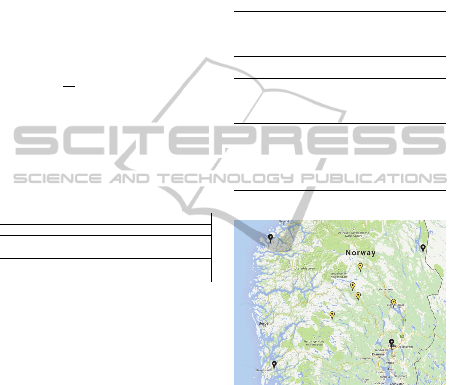
(1999). A 4-point grid with coarse spatial resolution
was built on the map of south of Norway.
Observation data from stations near and within the
grid points were used for training and verifying the
model. Four stations near the grid points were
chosen to be known stations and five stations within
the grid points were chosen to be unknown stations.
Figure 4 depicts our study area and the details of
these stations are presented in table 2.
For this study, we constructed feed-forward
networks which consist of three layers, one input
layer, one hidden layer and one output layer. There
were 9 neurons in the input layer, 10 neurons in the
hidden layer and one neuron in the output layer.
Usual root-mean-square error metric is defined as
the fitness function of our algorithm. The 9 variables
contained in the input layer are illustrated in table 3.
The output of the ANN is the maximum daily
temperature for an unknown station. An ANN was
built for each of the unknown stations.
Table 2: Study stations.
Station
Name Location
Known
station1
Fiskåbygd 62.10N, 5.58E
Known
station2
Nedre Vats 59.48N, 5.75E
Known
station3
Drevsjø 61.89N, 12.05E
Known
station4
Oslo Blindern 59.94N, 10.72E
Unknown
station1
Åbjørsbråten 60.92N, 9.29E
Unknown
station2
Løken I Volbu 61.12N, 9.06E
Unknown
station3
Kise Pa Hedmark 60.78N, 10.81E
Unknown
station4
Geilostølen 60.52N, 8.2E
Unknown
station5
Skåbu storslålen 61.52N, 9.38E
Figure 4: Map of study area. Black markers are known
stations and yellow markers are unknown stations.
3.1 Data Preparation
Maximum daily temperatures for a period from 1970
to 2010 were used for training and verifying our
model. Because not every day has valid data for all
stations due to some observation data missing, the
data was pre-processed and all data on invalid date
were removed. An invalid date defined in our
experiments is a day that anyone of the training
stations has missing data.
After pre-processing the dataset was shuffled
SIMULTECH2015-5thInternationalConferenceonSimulationandModelingMethodologies,Technologiesand
Applications
240

before presenting to ANN, in which 80% data were
randomly selected for training and 20% data were
selected for test. The reason to train our model with
shuffled data were two-fold: 1) the model we built in
this study is a spatial downscaling model, so to
present the training data with sequential order does
not make sense; 2) random ordering has been
reported to be superior to both sequential ordering
and aggregated values by Snell’s study (1999).
Table 3: Inputs of the NE model.
Input
number
Input
1 Maximum temperature at known station 1
2 Maximum temperature at known station 2
3 Maximum temperature at known station 3
4 Maximum temperature at known station 4
5 Distance between station 1 and unknown
station
6 Distance between station 2 and unknown
station
7 Distance between station 3 and unknown
station
8 Distance between station 4 and unknown
station
9 Elevation of unknown station
3.2 Experimental Results
We carried out 10 runs for training ANNs to learn
the relationship of maximum temperatures between
known stations and each of the unknown stations.
The average performance of each experiment took
about 400 to 600 seconds. Figure 5 shows average
learning curves of the ANNs from the 10 runs, and
table 4 shows our average test results.
From figure 5 we can see that the average RMSE
curves bend down very steeply in the first 100
generations, and then start coming down gently in
the rest of generations. As we introduced earlier,
EAs are optimal search algorithms. By integrating
EAs with ANNs, NE is able to find optimal
connection weights and topologies to map the
relationship of maximum temperatures between
knowns stations and unknown stations. The learning
curves shown in figure 5 indicate that our NE model
rapidly found relatively optimal connection weights
of ANNs at the early stages of evolution. After that
the NE model turned to gradually converge toward
global optima. Of course, NE algorithms cannot
guarantee to deliver the best ANN topology to a
problem, to find relatively optimal solutions,
however, are usually reachable.
Table 4: Overall performance measures. Average RMSE
and R
2
for test from 10 runs.
Station
RMSE R
2
Åbjørsbråten 2.91 0.898
Løken i Volbu 3.19 0.893
Kise Pa
Hedmark
2.85 0.912
Geilostølen 2.78 0.797
Skåbu
storslålen
2.79 0.911
Figure 5: Average learning curves of the ANNs from the
10 runs for the five unknown stations.
If we only measure the RMSE values shown in table
IV, the average RMSE achieved by our algorithms
are significantly smaller than those reported by some
other literatures (Snell et al., 1999; Cawley et al.,
2003; Coulibaly, 2004). However, to compare the
average R
2
values performed by our model with
those reported by others, our model does not appear
to be generally superior to other methods. Instead,
the average R
2
value for station Geilostølen is a bit
low. It is worthy of being mentioned, however, the
results reported in this paper were from the average
performance of our experiments. The compared
results from the above literatures were from the best
performance of their experiments.
In EAs, fitness functions play a crucial role to
guide how the evolutionary process goes to achieve
the objectives of problems. In our current NE
algorithm, only RMSE was considered in the fitness
function. The goal of our NE algorithm is, therefore,
merely to minimize RMSE values. However, a
smaller value of RMSE does not indicate a higher
value of R
2
. A possible improvement of our NE
2
3
4
5
6
7
0 100 200 300 400 500
Åbjørsbråten
Kise Pa Hedmark
Løken i Volbu
Geilostølen
Skåbu storslålen
Generations
RMSE (
o
C)
DownscalingDailyTemperaturewithEvolutionaryArtificialNeuralNetworks
241

model is to evolve ANNs by using multi-objective
evolutionary algorithms, which will be able to both
minimize the values of RMSE and maximize the
values of R
2
.
4 CONCLUSIONS
In this paper we have applied a NE model for the
spatial statistical downscaling of daily maximum
temperature. We demonstrated our approach by
interpolating temperature data from a large scaled
grid structure to interior points. The results of our
method showed good potential for the construction
of high-resolution scenarios. The future work of this
research can be comparison studies of our model
with the state of the art methods for the same study
area. In addition, our method can be improved by
using multi-objective evolutionary algorithms. Both
RMSE and R
2
should be taken into consideration
when we design the fitness function of the model.
ACKNOWLEDGEMENTS
The author would like to thank Rasmus Benestad
and Abdelkader Mezghani for valuable comments
and discussion.
REFERENCES
Brath, A., Montanari, A., and Toth, E., 2002, Neural
Networks and Non-parametric Methods for Improving
Realtime Flood Forecasting through Conceptual
Hydrological Models, Hydrology and Earth System
Sciences, vol. 6, pp. 627-640.
Bobbin, Jason and Yao, Xin, 1997, Solving Optimal
Control Problems with a Cost Changing Control by
Evolutionary Algorithms, Proceedings of
International Conference on Evolutionary
Computation, pp. 331-336.
Buche, D., Schraudolph, N. N., and Koumoutsakos, P.,
2005, Accelerating evolutionary algorithms with
Gaussian process fitness function models, IEEE
Transactions on Systems, Man, and Cybernetics, Part
C: Applications and Reviews, vol.35, no.2, pp.183-
194.
Carvalho, M. and Ludermir, T. B., 2006, Hybrid Training
of Feed-Forward Neural Networks with Particle
Swarm Optimization, Neural Information Processing,
vol. 4233, pp. 1061-1070.
Chadwick, R., Coppola, E., and Giorgi, F., 2011, An
artificial neural network technique for downscaling
GCM outputs to RCM spatial scale, Nonlinear
Processes in Geophysics, Vol. 18, No. 6, pp. 1013-
1028.
Coulibaly, Paulin, 2004, Downscaling daily extreme
temperatures with genetic programming, Geophysical
research letters, Vol 31, no. 16.
Cuéllar, M.P. and Delgado, M. and Pegalajar, M.C., 2006,
An Application of Non-linear Programming to Train
Recurrent Neural Networks in Time Series Prediction
Problems, Enterprise Information Systems VII, pp. 95-
102.
Dibike, Yonas B. and Coulibaly, Paulin, 2006, Temporal
neural netwroks for downscaling climate variability
and extremes, Neural Networks (Especial issue on
Earth Sciences and Environmental Applications of
Computational Intelligence), Vol. 19, No. 2, pp. 135-
144.
Downing, Keith L., 1997, The Emergence of Emergence
Distributions: Using Genetic Algorithms to Test
Biological Theories, Proceedings of the 7th
International Conference on Genetic Algorithms, pp.
751-759.
Eiben, A. E., Hinterding, R. and Michalewicz, Z., 1999,
Parameter control in evolutionary algorithms, IEEE
Transactions on Evolutionary Computation, vol.3,
no.2, pp.124-141.
Gavin C. Cawley, Malcolm Haylock, Stephen R. Dorling,
Clare Goodess and Philip D. Jones, 2003, Statistical
Downscaling with Artificial Neural Networks,
European Symposium on Artificial Neural Networks,
Bruges, pp. 167-172.
Hecht-Nielsen, R., 1989, Theory of the backpropagation
neural network, International Joint Conference on
Neural Networks, pp.593-605, vol.1.
Kohonen, T., Barna, G. and Chrisley, R., 1988, Statistical
pattern recognition with neural networks:
benchmarking studies, IEEE International Conference
on Neural Networks, pp.61-68.
Lu, Yingwei, Sundararajan, N. and Saratchandran, P.,
1998, Performance evaluation of a sequential minimal
radial basis function (RBF) neural network learning
algorithm,
IEEE Transactions on Neural Networks,
vol.9, pp.308-318.
Lubberts, Alex and Miikkulainen, Risto, 2001, Co-
Evolving a Go-Playing Neural Network, Proceedings
of GECCO San Francisco, pp. 14-19.
Moriarty, David E. and Miikkulainen, Risto, 1997,
Forming Neural Networks through Efficient and
Adaptive Coevolution, Evolutionary Computation,
vol. 5, pp. 373-399.
Regis, R. G. and Shoemaker, C. A., 2004, Local function
approximation in evolutionary algorithms for the
optimization of costly functions, IEEE Transactions
on Evolutionary Computation, vol.8, no.5, pp.490-
505.
Shi, Min, 2008, An Empirical Comparison of Evolution
and Coevolution for Designing Artificial Neural
Network Game Players, Proceedings of Genetic and
Evolutionary Computation Conference, pp. 379-386.
Snell, Seth E., Gopal, Sucharita and Kaufmann, Robert K.,
1999, Spatial Interpolation of Surface Air
SIMULTECH2015-5thInternationalConferenceonSimulationandModelingMethodologies,Technologiesand
Applications
242

Temperatures Using Artificial Neural Networks:
Evaluating Their Use for Downscaling GCMs, Journal
of Climate, vol. 13, pp. 886-895.
Specht, Donald F., 1991, A general regression neural
network, IEEE Transactions on Neural Networks,
vol.2, no.6, pp.568-576.
Stanley, Kenneth O. and Miikkulainen, Risto, 2002,
Evolving Neural Networks through Augmenting
Topologies, Evolutionary Computation, vol. 10 (2),
pp. 99-127.
Tsai, H. K., Yang, J. M., Tsai, Y. F., and Kao, C. Y., 2004,
An Evolutionary Algorithm for Large Traveling
Salesman Problems, IEEE Trans Syst Man Cybern B
Cybern, vol. 34, pp. 1718-1729.
Werbos, Paul J., 1974, Beyond Regression: New Tools for
Prediction and Analysis in the Behavioural Sciences,
Cambridge, Mass: Harvard University, 1974.
Xu, C. Y., 1999, From GCM to river flow: A review of
downscaling methods and hydrologic modeling, Prog.
Phys. Geogr., 23(2), pp. 229-249.
Yao, Xin, 1999, Evolving Artificial Neural Networks,
Proceedings of the IEEE, vol. 87, pp. 1423-1477.
Zerenner, Tanja, Venema, Victor, Friederichs, Petra and
Simmer, Clemens, 2014, Downscaling near-surface
atmospheric fields with multi-objective Genetic
Programming, Physics - Atmospheric and Oceanic
Physics, Computer Science - Neural and Evolutionary
Computing.
DownscalingDailyTemperaturewithEvolutionaryArtificialNeuralNetworks
243
