
A Notation for Discrimination Network Analysis
Fabian Ohler and Christoph Terwelp
Information Systems, RWTH Aachen University, Aachen, Germany
Keywords:
Rule-based Systems, Discrimination Networks.
Abstract:
Because of their ability to store, access, and process large amounts of data, Database Management Systems and
Rule-based Systems are used in many information systems as information processing units. A basic function
of a Rule-based System and a function of many Database Management Systems is to match conditions on
the available data. To improve performance intermediate results are stored in Discrimination Networks. The
resulting memory consumption and runtime cost depend on the structure of the Discrimination Network. A
lot of research has been done in the area of optimising Discrimination Networks. In this paper we focus on
re-using of network parts by multiple rule conditions. We introduce the block notation as a first step to enhance
optimisation. The block notation allows for the identification of meaningful sharing constructs.
1 INTRODUCTION
Because of their ability to store, access, and pro-
cess large amounts of data, Database Management
Systems and Rule-based Systems are used in many
information systems as information processing units
(Brownston et al., 1985; Forgy, 1981). A basic func-
tion of a Rule-based System and a function of many
Database Management Systems is to match condi-
tions on the available data. Checking all data repeat-
edly every time some data changes performs badly.
It is possible to improve performance by saving in-
termediate results in memory introducing the method
of dynamic programming. A common example for
this approach is the Discrimination Network. Differ-
ent Discrimination Network optimization techniques
are discussed in (Forgy, 1982), (Miranker, 1987), and
(Hanson and Hasan, 1993). These approaches only
address optimisations limited to single rules. Further
improvement is possible by optimising the full rule set
of a Rule-based System. In this paper we will intro-
duce a visualisable notation as a first step to enhance
optimisation of rule sets.
This paper is organized as follows: In Section 2
we introduce Discrimination Networks and in Sec-
tion 3 we explain the concept of re-using network
parts for different rules. In Section 4 we discuss the
arising problems in the field of node sharing. Those
problems are then addressed in Section 5 and the nota-
tion is presented. Section 6 comprises the conclusion
and gives an outlook on future work.
2 DISCRIMINATION NETWORKS
Rules in Rule-based Systems and Database Manage-
ment Systems both comprise a condition and actions.
The actions of a rule must only be executed, if the data
in the system matches the condition of the rule.
Discrimination Networks are an efficient method
of identifying rules to be executed employing dy-
namic programming trading memory consumption for
runtime improvements. Rule conditions are split into
their atomic (w. r. t. conjunction) sub-conditions. In
the following, such sub-conditions are called filters.
Discrimination Networks apply these filters suc-
cessively joining only the required data. Intermediate
Figure 1: Discrimination Network example.
566
Ohler F. and Terwelp C..
A Notation for Discrimination Network Analysis.
DOI: 10.5220/0005506205660570
In Proceedings of the 11th International Conference on Web Information Systems and Technologies (WEBIST-2015), pages 566-570
ISBN: 978-989-758-106-9
Copyright
c
2015 SCITEPRESS (Science and Technology Publications, Lda.)

results are saved to be reused in case of data changes.
Each filter is represented by a node in the Discrimina-
tion Network. Additionally, every node has a mem-
ory, at least one input, and one output. The mem-
ory of a node contains the data received via its inputs
matching its filter. The output is used by successor
nodes to access the memory and receive notifications
about memory changes. Data changes are propagated
through the network along the edges. Changed data
reaching a node is joined with the data saved in nodes
connected to all other inputs of the node. So only the
memories of affected nodes have to be adjusted. Each
rule condition is represented by a terminal node col-
lecting all data matching the complete rule condition.
An example Discrimination Network is shown in Fig-
ure 1.
data input nodes serve as entry points for specific
types of data into the Discrimination Network.
They are represented as diamond shaped nodes.
filter nodes join the data from all their inputs and
check if the results match their filters. They are
represented as inverted triangle shaped nodes.
terminal nodes collect all data matching the condi-
tions of the corresponding rules. They are repre-
sented as triangle shaped nodes. The action part
of a rule should be executed for each data set in
its terminal node.
3 NODE SHARING
The construction of a Discrimination Network that
exploits the structure of the rules and the facts to
be expected in the system is critical for the result-
ing runtime and memory consumption of the Rule-
based System. To avoid unnecessary re-evaluations
of partial results, an optimal network construction al-
gorithm has to identify common subsets of rule condi-
tions. In the corresponding Discrimination Network,
these common subsets may be able to use the output
of the same network nodes. This is called node shar-
ing.
Despite the fact, that there is a lot of potential
to save runtime and memory costs, current Discrimi-
nation Network construction algorithms mostly work
rule by rule. According to (The CLIPS Team, 1992)
the Rule-based System CLIPS tries to identify condi-
tion parts already present in the network for sharing.
The concept used in (Hanson and Hasan, 1993) also
mentions node sharing and the rating function used
to identify the best possible network assigns costs of
zero to network parts already present because of ear-
lier rules constructions. Taking the sharing of network
parts already constructed into consideration is a good
first step, but it will not always be possible to exploit
node sharing to its full extent. This is the case e. g.
if the nodes were constructed in a way, that the net-
work is (locally) optimal for the single rule it was con-
structed for, but prevents node-sharing w. r. t. further
rules and might therefore thwart finding the (globally)
optimal Discrimination Network for all rules in case
sharing the nodes would have reduced costs (cf. Ex-
emple 3.1).
Figure 2: Simple node sharing example network
Example 3.1. Assume there are two filters: filter f
1
uses facts of type a and b, filter f
2
uses facts of type b
and c. Furthermore there are two rules: rule r
1
using
f
1
and rule r
2
using f
1
and f
2
. Then filter f
1
is used
in both rules and we can construct a Discrimination
Network where both rules use the same node to apply
f
1
to the input (see Figure 2).
If we were to construct rule r
2
first and would have
decided to construct the node f
2
as an input for f
1
,
sharing f
1
with r
1
afterwards would have been im-
possible, since the output of the node for f
1
is also
already filtered by f
2
.
It is therefore advisable to construct the Discrimina-
tion Network, taking into account the set of rules as a
whole.
4 CHALLENGES
Since node sharing is beneficial in most situa-
tions, Discrimination Network construction algo-
rithms should be presented the necessary data to max-
imise the potential savings in runtime cost and mem-
ANotationforDiscriminationNetworkAnalysis
567
ory consumption. This section will present the chal-
lenges associated with generating these information.
Sadly, identifying common subsets of rule condi-
tions isn’t sufficient to make use of node sharing in
network construction. This can be seen by extending
the previous example.
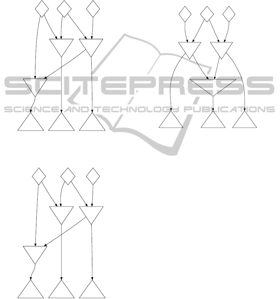
Figure 3: f
1
shared, twofold materialisation of f
2
.
Example 4.1. Assume there is an additional third rule
r
3
using only the filter f
2
. Now f
1
is part of r
1
and r
2
Figure 4: f
2
shared, twofold materialisation of f
1
.
while f
2
is part of r
2
and r
3
. Despite the fact that
there are two non-trivial rule condition subsets, we
can’t share both filters between the three rules in an
intuitive way. The rule r
2
requires a network that ap-
plies the filters f
1
and f
2
successively. Yet, the rule
r
1
(r
3
) needs the output of a node applying nothing
but f
1
( f
2
), meaning the corresponding nodes receive
unfiltered input. Thus, we need two nodes for the two
filters side by side at be beginning of the network and
some additional node to satisfy the chained applica-
tion of the two filters. There are three result networks
Figure 5: Sharing conflict solved using a special join.
still applying node sharing to some extent: We can
either share f
1
and duplicate f
2
(Figure 3), share f
2
and duplicate f
1
(Figure 4), or re-use both nodes for
r
2
by introducing an additional node that selects only
those pairs of facts that contain identical b-typed facts
in both inputs (Figure 5).
Formalising the phenomenon just observed, we say
that two filters are in conflict if they use the same
facts.
Employing the rating algorithm for discrimination
networks presented in (Ohler et al., 2013), we com-
pare the costs of the networks in Figure 5 and Fig-
ure 3. The memory consumption is the same in all sit-
uations, as the additional node always stores the same
data. To simplify matters, we ignored the effect of
paging and only inspected costs introduced by the in-
sertion of additional facts. The costs of fact deletions
look similar. Let c(b = b
0
) be the runtime cost for
the additional node in Figure 5 regarding insertions
and let c( f
0
1
) be the runtime cost for the additional f
1
node in Figure 4. Then
c(b = b
0
) − c( f
0
1
) = F
0
i
(b) ·
|
c
|
·
a on
f
1
b on
f
2
c
≥ 0
determines the additional costs needed for the node
b = b
0
not necessary for an additional f
1
node re-
garding fact insertions.
|
c
|
represent the estimated
fact count in the node c. F
0
i
(b) is an estimate for
WEBIST2015-11thInternationalConferenceonWebInformationSystemsandTechnologies
568

the frequency of fact insertions into the node b.
a on
f
1
b on
f
2
c
is an estimate for the number of facts
that match the two join predicates f
1
and f
2
. So, it
is never beneficial to use the network shown in Fig-
ure 5. The result looks analogue for an additional f
2
node. The choice between an additional f
1
or f
2
node
depends on the expected data, though.
5 BLOCK NOTATION
To ease the visualisation of conflict situations such as
the one described above and to allow for a straight-
forward network construction, we introduce a graph-
ical representation called the block notation. A block
in this notation consists of conflicting filters and rules
sharing those filters (i. e. the corresponding nodes).
Blocks are thus sets that are consistent in that all fil-
ters in a block are contained in all rules of the block
and all rules of the block contain all filters of the
block. As a start, we will only consider filters that
are in conflict with at most two other filters to allow
for two-dimensional diagrams.
filter
1 2
1
2
rule
Figure 6: Block diagram for Exemple 3.1.
Figure 6 shows the block diagram for Exem-
ple 3.1. The conflicting filters are shown as columns
in the grid and the conflicts are emphasised by the
|=
.
A dot on the grid indicates that a rule uses the corre-
sponding filter. The depicted block contains filter f
1
and the rules r
1
and r
2
suggesting the possibility to
share the filter between the two rules.
filter
1 2
1
2
3
rule
Figure 7: Block diagram for Exemple 4.1.
Figure 7 shows the block diagram for Exem-
ple 4.1. There are two blocks corresponding to the
previously identified common subsets of the rules.
The grey marker highlights the fact, that the blocks
touch each other implying that node sharing will re-
quire some form of special treatment.
We say that two blocks are in conflict if they touch
each other vertically or even overlap and it is not the
case that all filters of one of the blocks are contained
in the other block. Furthermore, a block set is com-
plete if no block is contained in another block and
for every rule there is one block containing all filters
of the rule. A block is maximal, if we can not add
another rule (because no further rule contains all the
filters in the block) or filter (because no further fil-
ter is contained in all the rules in the block) to it. To
further illustrate the block notation, we give another,
more complex example.
Example 5.1. Assume there are five filters f
1
, . . . , f
5
and three rules r
1
, r
2
, r
3
. Rule r
1
uses the first three
filters, r
2
uses all filters, r
3
uses the last three filters.
The filters f
i
and f
i+1
are in conflict for i = 1, . . . , 4.
This information is represented in Exemple 5.1. Ad-
filter
1 2 3 4 5
1
2
3
rule
Figure 8: Block diagram for Exemple 5.1 with maximal
blocks.
ditionally, all blocks of maximal size are depicted.
The given block set is complete, but there is one con-
flict in this block diagram: the top left 2 × 3 block is
in conflict with the bottom right 2 × 3 block.
filter
1 2 3 4 5
1
2
3
rule
Figure 9: Block diagram for Exemple 5.1 without conflicts.
A different (complete) set of blocks for the same
situation is shown in Figure 9. Choosing this par-
titioning produces no conflicts. Thus we can easily
translate it into a Discrimination Network. Figure 10
shows a possible result Discrimination Network leav-
ing out the nodes providing the facts for simplicity.
ANotationforDiscriminationNetworkAnalysis
569

Constructing the Discrimination Network for a
complete, conflict-free block set can be done by ma-
terialising the filters in the blocks starting with the
blocks containing the fewest filters. Within the set of
blocks containing an equal number of filters the order
is arbitrary, since none of these blocks can be the in-
put of another block in that set (otherwise they would
overlap and would have been in conflict).
The construction order is relevant only if blocks
contain the same filter-rule-combinations. Since the
blocks are conflict-free and the block set is complete,
if one block overlaps with another block, the filters
of one of the blocks are a subset of the filters of the
other block. As the one with fewer filters is con-
structed first, its output can be used to construct the
larger (w. r. t. filter count) block.
In Exemple 5.1, we start by constructing the filters
f
1
and f
3
for the 2 × 1 and the 3 × 1 block, respec-
tively. The next step is to add the filters f
2
using the
output of f
1
and f
3
for the 1 × 3 block and the filters
f
4
and f
5
in an arbitrary manner using the output of
f
3
for the 2 × 3 block. Finally, we add another f
2
for
the 1×5 block using the output of f
1
and the network
constructed for the 2 × 3 block.
Block diagrams become hard to draw and interpret
when filters are in conflict with more than two other
filters. The concept of blocks and conflicts remains
valid, though.
Figure 10: Possible result network for Figure 9.
6 CONCLUSION AND FUTURE
WORK
We presented the block notation as an abstraction to
share nodes and network parts. Using this notation we
defined the structure of meaningful sharing construc-
tions. The abstraction can be visualised in block di-
agrams (in a restricted form) easing the development
of algorithms to optimise node sharing.
Based on the notation presented, we are currently
developing optimisation algorithms considering sev-
eral rules at once. The output of such an algorithm
should be complete, conflict-free blocks. An optimis-
ing Discrimination Network construction algorithm
can then use this information to decide, whether node-
sharing is beneficial w. r. t. runtime cost and memory
consumption for the data to be expected. Develop-
ing such an algorithm with acceptable runtime costs
although it has to look at a set of rules instead of a
single one is pending.
REFERENCES
Brownston, L., Farrell, R., Kant, E., and Martin, N. (1985).
Programming expert systems in OPS5: an introduc-
tion to rule-based programming. Addison-Wesley
Longman Publishing Co., Inc., Boston, MA, USA.
Forgy, C. L. (1981). OPS5 User’s Manual. Technical report,
Department of Computer Science, Carnegie-Mellon
University.
Forgy, C. L. (1982). Rete: A fast algorithm for the many
pattern/many object pattern match problem. Artificial
Intelligence, 19(1):17 – 37.
Hanson, E. N. and Hasan, M. S. (1993). Gator : An Op-
timized Discrimination Network for Active Database
Rule Condition Testing. Tech. Report TR93-036, Univ.
of Florida, pages 1–27.
Miranker, D. P. (1987). TREAT: A Better Match Algorithm
for AI Production Systems; Long Version. Techni-
cal report, University of Texas at Austin, Austin, TX,
USA.
Ohler, F., Schwarz, K., Krempels, K.-H., and Terwelp, C.
(2013). Rating of discrimination networks for rule-
based systems. In DATA, pages 32–42.
The CLIPS Team (1992). Build Module. In CLIPS Archi-
tecture Manual, pages 143–147.
WEBIST2015-11thInternationalConferenceonWebInformationSystemsandTechnologies
570
