Experimental Modal Analysis based on a Gray-box Model of Flexible

Structures

Alberto Cavallo

, Giuseppe De Maria

, Michele Iadevaia

, Ciro Natale

and Salvatore Pirozzi

Seconda Universit`a di Napoli, Dip. di Ingegneria Industriale e dell’Informazione, Via Roma 29, 81031 Aversa, Italy

Dynamic Design Solutions (DDS) NV, Leuven, Belgium

Keywords:

Experimental Modal Analysis, Subspace Identiﬁcation, Flexible Structures.

Abstract:

The main objective of this paper is to propose an experimental modal analysis procedure, based on the use of

a gray-box model for ﬂexible structures. The described approach presents interesting advantages with respect

to commercial solutions: ease of use due to the low number of parameters to set for an identiﬁcation session;

no need for expert users, even in the presence of particular cases such as double modes, since it does not use

a stabilization diagram to be elaborated; use of a gray-box model whose unknown parameters have a clear

physical meaning. All these characteristics are discussed in the paper, and the performance of the proposed

procedure has been evaluated by using experimental data available from a non-trivial standard benchmark.

The results have been compared with those obtained by using a commercial tool.

1 INTRODUCTION

Experimental modal analysis has become a key tech-

nology in structural dynamic analysis and in mechan-

ical products development. Modal analysis is the pro-

cess of extracting the dynamics characteristics of a vi-

brating system from experimental data (Ewins, 1984).

When all of these parameters have been obtained, a

complete mathematical model of the system can be

deﬁned. The mathematical model may then be used

in computer simulations to predict the response of the

system when it is modiﬁed, so that a designer can

evaluate different design modiﬁcations without build-

ing prototypes (Ewins, 1984; Heylen et al., 1995) or

to design an active vibration and noise control for a

ﬂexible structure (Cavallo et al., 2008; Cavallo et al.,

2010).

This paper presents a new frequency domain pro-

cedure for experimental modal analysis, based on the

use of a gray-box model of ﬂexible structures. The

main objective of the paper is to show how, with the

proposed approach, it is possible to obtain experimen-

tal results similar to those obtained with the commer-

cial solutions, but with some advantages in terms of

experience required to the user and physical mean-

ing of the model unknown parameters. The procedure

uses the results of the identiﬁcation method proposed

in (Cavallo et al., 2007). Differently from (Cavallo

et al., 2007), where the identiﬁcation procedure was

developed only for model-based control applications,

in this paper for the ﬁrst time the same procedure has

been adapted, as regards the estimation of the mode

shapes, for experimental modal analysis. The pro-

posed procedure is compared with the polyreference

Least Squares Complex Frequency domain method

(pLSCF) (Guillaume et al., 2003). The comparison

is made with this algorithm since the pLSCF is one of

newest approach presented in literature and moreover

there are some papers in which the pLSCF is com-

pared with the others classical methods (Guillaume

et al., 2003; Peeters et al., 2004), obtaining an indirect

comparison also with these last ones. The pLSCF al-

gorithm has been applied by using the modal analysis

estimator module integrated in the commercial soft-

ware FEMtools

(FEMtools Version 3.6, 2012).

The proposed procedure, similarly to the pLSCF

method, separates the estimation of the system poles

from the mode shapes. However, the pLSCF method

uses a polynomial form and generally it starts with a

model order very high, trying to ﬁt models that con-

tain much more modes than those actually present in

the experimental data. Then, the true physical modes

are separated from the spurious ones by interpret-

ing the so-called ”stabilization diagram” by an expert

user. The poles corresponding to a certain model or-

der are compared to the poles of a one order lower

model and if their differences are minor than pre-set

limits, the pole is labelled as a stable one. The spu-

439

Cavallo A., De Maria G., Iadevaia M., Natale C. and Pirozzi S..

Experimental Modal Analysis based on a Gray-box Model of Flexible Structures.

DOI: 10.5220/0005504304390447

In Proceedings of the 12th International Conference on Informatics in Control, Automation and Robotics (ICINCO-2015), pages 439-447

ISBN: 978-989-758-122-9

 2015 SCITEPRESS (Science and Technology Publications, Lda.)

rious poles will not be stable during this comparison

and will be sorted out of the modal parameters. Fi-

nally, an eigenvalue decomposition of the companion

matrix, associated with the polynomial coefﬁcients

identiﬁed, is implemented to compute the real modal

parameters (Guillaume et al., 2003). The number of

parameters to set by the user before starting the op-

timization procedure is high and can lead to wrong

results if the user experience is not adequate.

Differently from the commercial solutions, the

procedure here proposed estimates the eigenvalues by

using a subspace approach, and the user is required

only to ﬁx the number of modes to identify and to

select the frequency range in which to perform the

identiﬁcation. Spurious modes outside the frequency

range of interest are not extracted. Moreover, the pro-

posed approach does not use a stabilization diagram

to select stable poles in the selected frequency range,

since the stability of the estimated poles is guaran-

teed by the identiﬁcation procedure of the dynamic

matrix detailed in (Cavallo et al., 2007). As a conse-

quence, the interaction of an expert user is not nec-

essary, even in the presence of particular cases such

as double modes. This feature makes the proposed

approach very interesting to be automated for applica-

tions where iterative modal analysis is necessary (e.g.,

health monitoring, model-based control, optimal po-

sitioning of actuators and sensors for control).

Another advantage of the proposed procedure is

the use of a gray-box model whose unknown param-

eters have a clear physical meaning. In particular, for

all the applications where a numerical–experimental

correlation between a ﬁnite element model and exper-

imental data is necessary, the use of a gray-box model

can simplify the user task of tuning the numeric pa-

rameters in order to match the experimental data.

2 MODELLING OF FLEXIBLE

STRUCTURES

Consider a n−degree-of-freedom mechanical system

whose generalized coordinates are represented by a

n× 1 vector q and with n×n mass matrix M and stiff-

ness matrix K; both matrices are positive deﬁnite and

symmetric. The equation of motion can be written in

the form (Cavallo et al., 2010)

M ¨q+ Kq = f (1)

where f is the n× 1 vector of generalized forces. It is

evident that the state of this dynamic system is con-

stituted by the 2n × 1 vector z = (q

˙q

)

. With this

choice, the state space representation of the system is

˙z =



0 I

−M

−1

K 0





−1



y = (0 I)z

if the observed output is the velocity ˙q. Since the ma-

trix M

−1

K have all real and positive eigenvalues, it

can be diagonalized by solving the following eigen-

value problem

−1

KU = UΩ (2)

where Ω = diag{ω

,... ,ω

} is the diagonal matrix

of the eigenvaluesof M

−1

K andU is the matrix whose

columns are the eigenvectors of M

−1

K, the so-called

“mode shapes”. It is well-known that the eigenvectors

are orthogonal with respect to the mass matrix and

thus they can be normalized so as

MU = I (3)

Now, deﬁne the transformation in the state space

z =



U 0

0 U



x, (4)

where x are the so-called “modal coordinates”, and

consider a number m of input forces f

, i ∈ F ⊆

{1,. .. ,m} applied to the structure along a set of de-

grees of freedom, so that, deﬁning the unit vector e

as the vector with 1 at entry i and 0 elsewhere, a se-

lection matrix S can be deﬁned whose rows are e

i ∈ F . Assuming to observe the velocity along the

same degrees of freedom, the state space representa-

tion assumes the form

˙x = Ax + Bu =



0 I

−Ω −Λ







f (5)

y = Cx = (0 SU)x (6)

where the diagonal matrix Λ =

diag{2ζ

,... ,2ζ

}, being ζ

∈ (0,1) the

damping coefﬁcient of the i−th mode, has been

introduced to take into account the unavoidable

damping present in the physical system. Notice, that

this corresponds to add in Eq. (1) the friction forces

d = D ˙q acting in the material, with a proportional

damping matrix D = α

K + α

M. This choice to add

a proportional damping in the model Eq. (1) changes

the ﬁnite-dimensional, complex eigenvalue problem.

In particular, the solution yields n pairs of complex

conjugate eigenvalues, named “modes”

= −ζ

± jω

1− ζ

i = 1, ...,n (7)

where λ

is the i−th complex eigenvalue of the struc-

ture. The Eq. (7) represents the relation between the

ICINCO2015-12thInternationalConferenceonInformaticsinControl,AutomationandRobotics

440

complex eigenvalue, the damping coefﬁcient ζ

and

the natural frequency ω

of the i−th mode.

Furthermore, this choice for the viscous damping

has also the following implications: it does not affect

the mode shapes that are the eigenvectors (ψ

∈ C

)

of the matrix M

−1

K; the mode shapes are real and or-

thonormal; each mode shape is described by a stand-

ing wave that contains ﬁxed stationary node points.

In contrast, if the matrix D is not representative of a

proportional damping, the mode shape are complex

valued and results in modes, which are described as

complex modes, having different characteristics; each

mode shape is described by a travelling wave and ap-

pears to contain a moving node point on the struc-

ture; in such a case, the mode shape from the un-

damped case does not diagonalise the damping matrix

D. Since in the typical case of experimental modal

analysis the available data are Frequency Response

Functions (FRFs), also the relations between the gray-

box model and the FRFs data are useful. In particu-

lar, applying the Fourier transform, the frequency re-

sponse matrix corresponding to the model (5)–(6), is

symmetric and has the form

G( jω) = UΦ( jω)U

(8)

with Φ( jω) = diag{φ

( jω),. .. , φ

( jω)} and

( jω) = jω/(ω

− ω

+ j2ζ

ω), l = 1,. .., n

and thus for an applied force at a spatial position k

(as input) and a velocity measurement at a spatial

position h (as output), the FRF g

( jω) in physical

coordinates is

( jω) =

∑

l=1

( jω)ψ

(9)

where ψ

is the h-th column of the matrix U of the

mode shape corresponding to the l-th mode.

3 MODAL PARAMETERS

ESTIMATION

The objective of experimental modal analysis (Ewins,

1984) is to derive natural frequencies and damping

coefﬁcients as well as mode shapes. In the proposed

approach, the unknown parameters to identify are ex-

plicitly present in the gray-box model reported in

Eqs. (5)–(6) and used in the identiﬁcation procedure.

Note that if the number of excitation inputs is differ-

ent from the number of measured outputs, the selec-

tion matrix in Eq. (5) is different from the one in the

Eq. (6). In particular, if the number of inputs is equal

to m and the number of outputs is p (p > m is the typi-

cal case of experimental modal analysis) the gray-box

model can be rewritten as

˙x =



0 I

−Ω −Λ







u (10)

y =



0 C



x (11)

where Λ,Ω ∈ R

n×n

, B

∈ R

n×m

and C

∈ R

p×n

have

to be estimated. With this choice, the rows of B

represent spatial samples of the mode shapes corre-

sponding to excitation points, while the columns of

represent spatial samples of the mode shapes cor-

responding to measurement points.

All the parameters to be identiﬁed for the

model (10)–(11) can be estimated by using the pro-

cedure detailed by the same authors in (Cavallo et al.,

2007). The only choices that the user has to do, as dis-

cussed in the introduction, are: to select the frequency

range in which to perform the identiﬁcation and to ﬁx

the number of modes to identify.

The selection of the working frequency range

[ f

, f

]Hz, in which to extract the modes of interest,

has to take into account that the real system is inﬁ-

nite dimensional. In fact, for ﬂexible structures the

FRFs in a given frequency range depend not only on

the modes with natural frequencies within the con-

sidered range but also on the lower and higher fre-

quency modes. This means that near the extremes

of the range the experimental data are not sufﬁcient

for an accurate identiﬁcation of modal parameters and

thus the FRFs should be measured on a working fre-

quency range [ f

′

, f

′

]Hz wider than the interesting one

[ f

′

, f

′

] ⊃ [ f

, f

]. Fixed the frequency range, denote

with G

∈ C

p×m

, i = 1, .. .,M the experimentalmea-

sured samples of the frequency response matrix in the

frequency range [ f

′

, f

′

]Hz (not necessarily uniformly

spaced). The choice of M depends on the modal

density of the ﬂexible structure and obviously on the

width of the frequency range of interest. The num-

ber of the modes to be identiﬁed (n) can be ﬁxed on

the basis of a classical indicator used in experimental

modal analysis (Ewins, 1984), i.e.

H(ω

) =

∑

h=1

∑

k=1

( jω

)|, i = 1,. .., M (12)

by counting (approximately and lightly overestimat-

ing) its number of peaks by simple inspection.

By following the procedure in (Cavallo et al.,

2007), in a ﬁrst step, the M measured samples of the

FRFs are used to construct the matrices detailed in

the cited paper, from which, via a subspace identiﬁca-

tion technique, the eigenvalues of the dynamic matrix

A are estimated. At the end of this step, the n ﬁxed

modes are completely estimated in terms of natural

frequencies and damping ratios. The second stage

consists in determining an estimate of B

and C

. In

ExperimentalModalAnalysisbasedonaGray-boxModelofFlexibleStructures

441

particular, in view of (9), the frequency response ma-

trix can be written as

G( jω) =

∑

l=1

( jω)c

∑

l=1

( jω)R

(13)

where R

= c

∈ R

p×m

is the residue matrix corre-

sponding to the l-th mode, with c

and b

the l-th col-

umn of C

and the l-th row of B

, respectively. From

Eq. (13) it is evident that the unknown parameters R

can be easily computed by resorting to a least mean

square technique, being G( jω) the measured data and

the generic φ

( jω) known from the ﬁrst step. From

the estimated R

residues it is possible to construct the

matrices B

and C

in different ways. The interested

reader can refer to (Cavallo et al., 2007) and (Cavallo

et al., 2010) for more details. For the experimental

modal analysis, objective of this paper, the estima-

tion of residues is sufﬁcient. In fact, the estimated

residues allows an easy estimation of the so called

modal constants from which any normalization can

be chosen to estimate the mode shapes (details can be

found in any textbook on experimental modal analy-

sis, e.g., (Ewins, 1984; Heylen et al., 1995)). Recall-

ing that the modal constants are the constant matrices

appearing in the following decomposition of the

FRF matrix

G( jω)=

∑

l=1

( jω)R

= jω

∑

l=1



jω − λ

∗

jω − λ

∗



(14)

it is straightforward to see that the modal constants

are related to the residues as

2jω

1− ζ

. (15)

Equation (15) shows the classical property that modal

constants are purely imaginary for ﬂexible structures

exhibiting only stationary waves. For the evaluation

of the experimental results in the remainder of the pa-

per, the normalization selected to compute the nor-

malized mode shape from the modal constant, corre-

sponding to the l-th mode, is

Im(A

)

max|(A

. (16)

4 EXPERIMENTAL RESULTS

The proposed approach for the experimental modal

analysis has been tested by using data for the Modal

Parameter Estimation (MPE) Round Robin. This

round robin is an initiative of the Michigan State

Technical University (MTU) and was presented at the

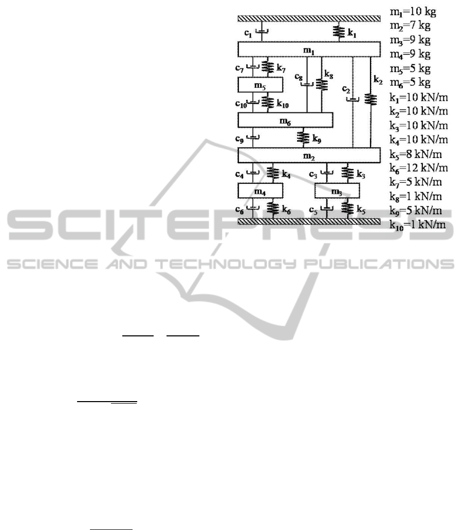
Figure 1: Lumped parameter model used to generate cali-

bration data set for IMAC MPE Round Robin.

recent IMAC XXIX conference. More than twenty

participants from several countries has taken part in

the exercise, performed on simulated and experimen-

tal data. The data are available for research activities

on the web (IMAC website, 2011). In particular, the

calibration data set with proportional damping and the

experimental data of the plexiglass plate available on-

line have been considered for this work. For each data

set a comparison with the FEMtools

commercial

solution is also presented.

4.1 The Calibration Data

The calibration data sets, available from IMAC MPE

Round Robin, were generated using a lumped pa-

rameters model, constituted by 6 masses, 10 springs

and 10 dampers. The details about the model are re-

ported in Fig. 1 (see also the web site (IMAC website,

2011)). As detailed above, the proposed approach is

based on a gray-box model with proportional damp-

ing. According to this hypothesis, the data set with

D = 0.0001K + 0.05M has been selected. As de-

scribed above, the only choice, that the proposed ap-

proach asks the user, is to set the number n of modes

to identify. For a lumped parameter model the num-

ber of mode is ﬁnite, and in particular is n = 6 for

the selected model. With this choice of n, the pro-

posed approach has been applied, starting from the

FRF samples of the considered calibration data set, to

estimate the modal parameters of the lumped param-

eter model. The results are reported in Table 1, where

ICINCO2015-12thInternationalConferenceonInformaticsinControl,AutomationandRobotics

442

Table 1: Calibration data with proportional damping: modes extracted by using the proposed approach.

Mode # ω

[Hz] ω

[Hz] E

[%] ζ

[%] E

[%] MAC

alias [%] MAC

[%]

1 3.395 3.506 3.269 0.224 0.224 0 3.25 99.67

2 5.238 5.493 4.868 0.240 0.245 2.083 2.72 98.13

3 6.423 6.427 0.062 0.264 0.264 0 3.05 99.84

4 7.547 7.552 0.066 0.290 0.290 0 0.51 99.86

5 8.305 8.388 0.999 0.309 0.311 0.647 3.25 98.78

6 12.639 12.641 0.016 0.428 0.429 0.234 1.03 99.98

the natural frequencies and the damping ratios of the

estimated modes are compared to the actual ones, an-

alytically obtained by the numeric matrices M, K and

D. The percentage errors for the estimated natural fre-

quencies have been quantiﬁed as

|ω

− ω

100, (17)

where ω

and ω

are the actual and the estimated val-

ues of the natural frequencies, respectively. Similarly,

for the damping ratios the following percentage error

has been evaluated

|ζ

− ζ

100, (18)

where ζ

and ζ

represent the actual and the estimated

values of the damping ratios, respectively. The re-

sults, reported in Table 1, show the good estimation

obtained for all the 6 modes of the considered model.

The percentage errors are always less than 5% and of-

ten less than 1%. For the mode shapes, the results

have been evaluated by using the classical Modal As-

surance Criterion (MAC). The MAC index between

two modes ψ

and ψ

is deﬁned as:

MAC =

|ψ

(ψ

)(ψ

)

100, (19)

where the symbol (·)

indicates the transpose con-

jugate. The MAC index can be used to evaluate the

correlation between: two mode shapes of the same

estimated model; an estimated mode shape with the

corresponding actual mode shape; two corresponding

100

Mode #

MAC [%]

Figure 2: Calibration data with proportional damping:

MAC

for the modes extracted with the proposed approach.

mode shapes estimated by using two different proce-

dures. Based on this observations, the ﬁrst signiﬁ-

cant analysis is the evaluation of the correlation be-

tween the mode shapes of the estimated model. In

particular, since the mode shapes deﬁne an orthogo-

nal basis, they are uncorrelated and the correspond-

ing MAC value should be zero. As a consequence,

computing the MAC values for a set of mode shapes

of the same model should, in theory, provide a diag-

onal matrix, i.e. diagonal elements with a value of

100 and zero-valued off-diagonal elements. Hence,

the MAC

index values have been computed by using

Eq. (19), where ψ

and ψ

(with i, j = 1, .. .,6) are the

normalized mode shape obtained from Eq. (16). The

results are reported in Fig. 2, where the off-diagonal

elements are clearly very low. The maximum MAC

alias, which is the highest off-diagonal value for the

considered modes, is reported in Table 1 to simplify

its evaluation. The comparison of the estimated mode

shapes with the actual ones, analytically obtained by

the numeric matrices M, K and D, has been carried

out by computing the MAC

index values by using

Eq. (19). In particular, the correlation between the es-

timated ψ

and the corresponding actual ψ

normal-

ized mode shapes (with i = j = 1, ...,6) has been

computed for the 6 modes of the considered model.

The excellent results are reported in the last column

of Table 1. In order to better appreciate the results

obtained with the proposed approach, the MPE has

been also carried out by using the commercial solu-

tion FEMtools

. The same calibration data have

been used to implement the same analysis. Hence, the

same experimental results are reported to allow a fair

100

Mode #

MAC [%]

Figure 3: Calibration data with proportional damping:

MAC

for the modes extracted by using FEMtools.

ExperimentalModalAnalysisbasedonaGray-boxModelofFlexibleStructures

443

Table 2: Calibration data with proportional damping: modes extracted by using FEMtools.

Mode # ω

[Hz] ω

[Hz] E

[%] ζ

[%] E

[%] MAC

alias [%] MAC

[%]

1 3.395 3.506 3.269 0.224 0.224 0 3.21 99.67

2 5.238 5.493 4.868 0.240 0.245 2.083 2.69 98.14

3 6.423 6.427 0.062 0.264 0.264 0 3.06 99.84

4 7.547 7.552 0.066 0.290 0.290 0 0.49 99.86

5 8.305 8.388 0.999 0.309 0.311 0.647 3.21 98.78

6 12.639 12.641 0.016 0.428 0.428 0 1.00 99.99

comparison. The estimated natural frequencies and

damping ratios have been compared with the actual

ones and the mode shapes have been evaluated by us-

ing the MAC indices. The corresponding results are

reported in Table 2 and Fig. 3. The obtained results

are practically identical. These results, obtained in a

standard benchmark, allow to conclude that the pro-

posed method is technically sound and with the same

performance of a well assessed method, but with the

advantage that the number of parameters to set for an

identiﬁcation procedure is lower than a commercial

solution since this procedure does not use a stabiliza-

tion diagram.

4.2 The Plexiglass Plate

The plexiglass plate data, available from IMAC MPE

Round Robin, were acquired from a plexiglas plate

that measures 53 × 32× 1.5cm. The plexiglass mate-

rial has been chosen in order to obtain high damped

modes. The plate has been designed to have a dou-

ble mode at the ﬁrst resonance peak in order to obtain

non-trivial experimental data. The identiﬁcation of

these double mode is the greater difﬁculty on which

to assess the performance of the proposed approach.

The plate was tested in a free-free boundary condi-

tion. The measurements were made by using triaxial

accelerometers, mounted with the wax and a random

excitation signal as source. Hence, the available FRF

data have accelerations as outputs and forces as in-

puts. Since the proposed approach uses a gray-box

100

Mode #

MAC [%]

Figure 4: Plexiglass plate data: MAC

for the modes ex-

tracted by using the proposed approach.

model with velocities as outputs, a preliminary divi-

sion by jω has been applied to the data in order to

compute the necessary FRF samples. The proposed

approach has been applied by ﬁxing the number of

modes n = 20, by using the indicator in Eq. (12). The

ﬁrst 10 extracted modes are reported in Table 3. In

particular the natural frequencies and the damping ra-

tios are reported in the ﬁrst two columns. Concerning

the mode shapes, as made for the calibration data, the

MAC

index has been evaluated for the 10 identiﬁed

modes and the results are reported in Fig. 4, while the

MAC

alias values are reported in the 4-th column of

the Table 3. In this case, since no actual values are

available, only a comparison with the results carried

out by using FEMtools is possible. The results about

the ﬁrst 10 modes extracted with the commercial tool

are reported in Table 4 and in Fig. 5. In this experi-

mental case, the differences between the proposed ap-

proach and the commercial solution are very low, in

terms of natural frequencies and damping ratios for

the extracted modes. Concerning the mode shapes,

separate discussions for the ﬁrst two modes, that rep-

resent the double mode, and the remaining ones have

to be done. In particular, Fig. 4 shows that the mode

shapes associated to the ﬁrst two modes, evaluated

by using the proposed approach, are clearly two dis-

tinct modes, since the MAC

index between mode 1

and mode 2 is about 7%. Instead, from Fig. 5, it is

evident that the ﬁrst two modes, evaluated by using

FEMtools, are more similar to each other, showing a

MAC

index between them of about 28%. For the re-

Table 3: Plexiglass plate: ﬁrst 10 modes extracted by using

the proposed approach.

Mode # ω

[Hz] ζ

[%] MAC

alias [%] MAC

[%]

1 99.660 4.85 7.8 69.23

2 99.717 6.07 14.7 71.25

3 226.792 3.66 10.7 97.88

4 279.570 3.53 3.3 92.30

5 291.574 3.48 8.5 94.30

6 356.267 3.25 8.6 96.77

7 417.760 3.36 14.7 93.81

8 502.296 3.03 25.9 82.95

9 569.037 3.01 11.2 88.72

10 667.035 4.07 34.34 56.10

ICINCO2015-12thInternationalConferenceonInformaticsinControl,AutomationandRobotics

444

100

Mode #

MAC [%]

Figure 5: Plexiglass plate data: MAC

for the modes ex-

tracted by using FEMtools.

maining modes, the differences between the proposed

approach and FEMtools in terms of MAC

and MAC

alias, are not signiﬁcant since the MAC index values

are sometimes in favor of the proposed approach and

other in favor of the commercial tool, but always suf-

ﬁciently low. It is important to remark that the ex-

traction of the double mode, by using FEMtools, has

required iterated attempts by an expert user. With-

out the expertise there is the risk of confusing, dur-

ing the identiﬁcation procedure, the double mode with

a simple mode. On the contrary, with the proposed

approach, there are not differences due to the pres-

ence/absence of double modes. An additional MAC

index has been computed by using Eq. (19) to evaluate

the correlation between the ψ

and the corresponding

normalized mode shapes (with i = j = 1,. ..,10),

estimated with the proposed approach and the com-

mercial tool, respectively. These correlation index

values, computed for the ﬁrst estimated 10 modes, are

reported in the last column of the Table 3. The results

show that the mode shapes #1, #2 and #10 have dis-

crete differences.

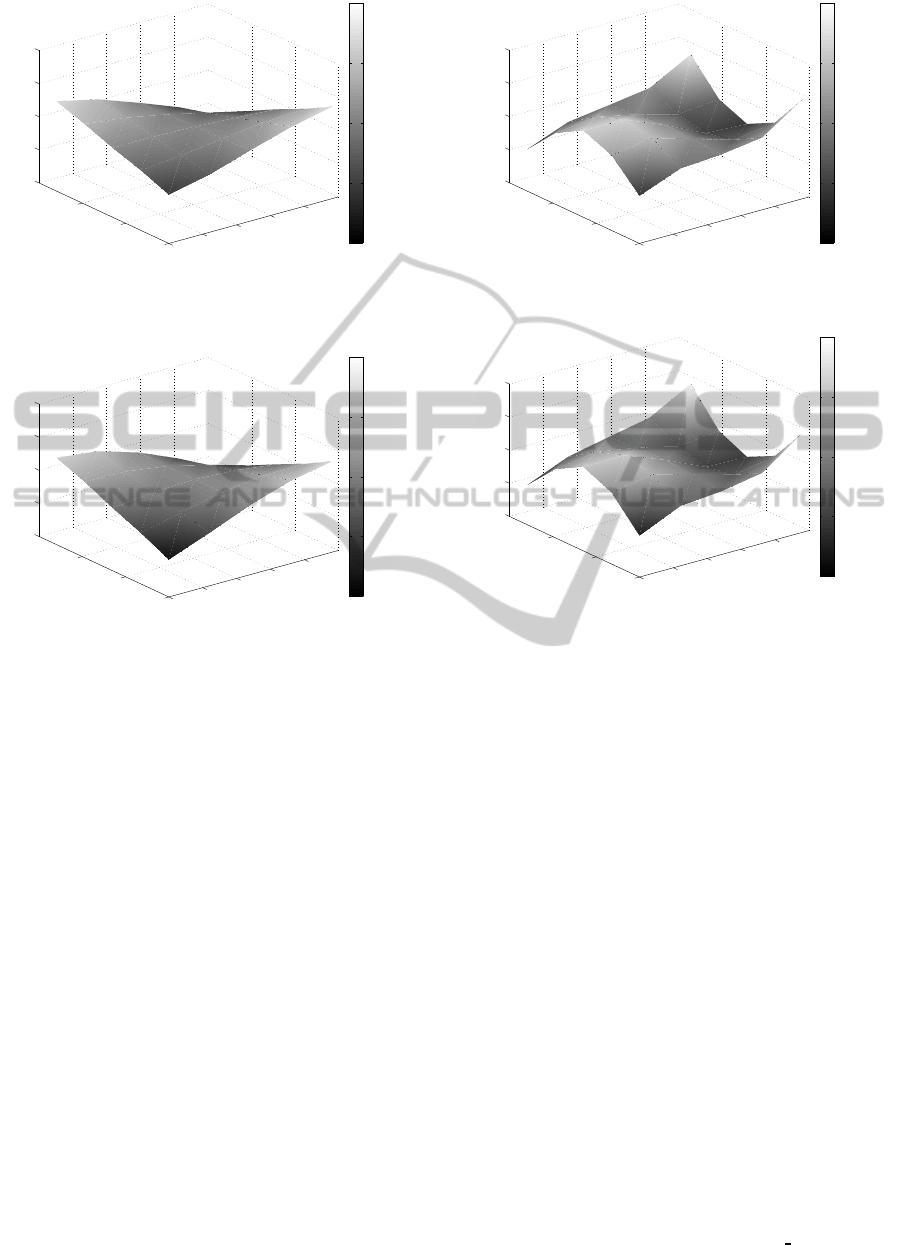
To further highlight the quality of the results

obtained, the spatial reconstruction of some mode

shapes are reported, both for the proposed approach

Table 4: Plexiglass plate: ﬁrst 10 modes extracted by using

FEMtools.

Mode # ω

[Hz] ζ

[%] MAC

alias [%]

1 99.917 4.53 28.18

2 100.130 4.80 28.18

3 226.633 3.71 12.2

4 279.301 3.70 28.2

5 290.900 3.44 6.1

6 355.853 3.40 34.3

7 417.651 3.24 35.1

8 503.163 3.25 4.5

9 568.682 2.93 10.1

10 672.990 3.17 23.3

0.1

0.2

0.3

0.4

0.1

0.2

−2

−1

x [m]

y [m]

normalized z

−1

−0.5

0.5

Figure 6: Plexiglass plate data: normalized mode shape

at 99.660 Hz (Mode #1), estimated with the proposed ap-

proach.

and the commercial solution. First off all, the mode

shapes associated to the double mode are reported,

since they represent the more interesting problem for

the considered experimental data. In particular, Fig. 6

and 8 reports the normalized mode shapes for the dou-

ble mode, obtained with the proposed approach, while

Fig. 7 and 9 the corresponding mode shapes, obtained

with FEMtools

An additional mode shape for the remaining

modes is reported for completeness of the work. In

particular, Fig. 10 and 11 show the normalized mode

shapes corresponding to mode #6. From the MAC in-

dex values reported in previous tables it is evident that

the quality of all other modes is very similar to that of

the mode #6 here plotted.

5 CONCLUSIONS

In this paper an experimental modal analysis, based

on the use of a gray-box model, has been presented.

A ﬁrst advantage of the proposed approach is the low

number of parameters needed to be set: the user is

required only to ﬁx the number of modes to identify

0.1

0.2

0.3

0.4

0.1

0.2

−2

−1

x [m]

y [m]

normalized z

−1

−0.5

0.5

Figure 7: Plexiglass plate data: normalized mode shape at

99.917 Hz (Mode #1), estimated by using FEMtools.

ExperimentalModalAnalysisbasedonaGray-boxModelofFlexibleStructures

445

0.1

0.2

0.3

0.4

0.1

0.2

−2

−1

x [m]

y [m]

normalized z

−1

−0.5

0.5

Figure 8: Plexiglass plate data: normalized mode shape at

99.717 Hz (Mode #2), estimated by using the proposed ap-

proach.

0.1

0.2

0.3

0.4

0.1

0.2

−2

−1

x [m]

y [m]

normalized z

−1

−0.5

0.5

Figure 9: Plexiglass plate data: normalized mode shape at

100.130 Hz (Mode #2), estimated by using FEMtools.

and to select the frequency range in which to perform

the identiﬁcation. Moreover, the proposed approach

does not use a stabilization diagram to select stable

poles in the selected frequency range and, as a con-

sequence, the interaction of an expert user is not nec-

essary, even in the presence of particular cases such

as double modes. Another advantage of the proposed

procedure is the use of a gray-box model whose un-

known parameters have a clear physical meaning: for

all the applications where a numerical–experimental

correlation between a ﬁnite element model and exper-

imental data is necessary, the use of a gray-box model

can simplify the user task of tuning the numeric pa-

rameters in order to match the experimental measure-

ments. The experimental results, obtained in a stan-

dard benchmark, are practically identical to those ob-

tained with commercial solutions, with some advan-

tages for double mode identiﬁcation. These results

allow to conclude that the proposed method is techni-

cally sound and with the same performance, of a well

assessed method, but with the advantages just summa-

rized. Future activities are planned in order to test the

proposed approach to more complex ﬂexible systems.

0.1

0.2

0.3

0.4

0.1

0.2

−2

−1

x [m]

y [m]

normalized z

−1

−0.5

0.5

Figure 10: Plexiglass plate data: normalized mode shape at

356.267 Hz estimated by using the proposed approach.

0.1

0.2

0.3

0.4

0.1

0.2

−2

−1

x [m]

y [m]

normalized z

−1

−0.5

0.5

Figure 11: Plexiglass plate data: normalized mode shape at

355.853 Hz estimated by using FEMtools.

REFERENCES

Cavallo, A., De Maria, G., Natale, C., and Pirozzi, S.

(2007). Gray-box identiﬁcation of continuous-time

models of ﬂexible structures. IEEE Trans Contr Syst

Tech, 15:967–981.

Cavallo, A., De Maria, G., Natale, C., and Pirozzi, S.

(2008). Robust control of ﬂexible structures with sta-

ble bandpass controllers. Automatica, 44:1251–1260.

Cavallo, A., De Maria, G., Natale, C., and Pirozzi, S.

(2010). Active Control of Flexible Structures–From

modelling to implementation. Springer, London.

Ewins, D. (1984). Modal Testing: Theory and Practice.

Research Studies Press LTD, Baldock.

FEMtools Version 3.6 (2012). Dynamic Design Solutions.

(www.femtools.com), Leuven, Belgium.

Guillaume, P., Verboven, P., Vanlanduit, S., Van der Auwer-

aer, H., and Peeters, B. (2003). A poly-reference im-

plementation of the least-squares complex frequency-

domain estimator. In Proc. of International Modal

Analysis Conference (IMAC XXI), Kissimmee, FL.

Heylen, W., Lammens, S., and Sas, P. (1995). Modal Anal-

ysis Theory and Testing. Department of Mecanical

Engineering, Katholike Universiteit Leuven, Leuven.

IMAC website (2011). www.me.mtu.edu/imac

mpe/. Modal

ICINCO2015-12thInternationalConferenceonInformaticsinControl,AutomationandRobotics

446

Parameter Estimation Round Robin, Int. Modal Anal-

ysis Conf. (IMAC XXIX), Jacksonville, FL.

Peeters, B., Guillaume, P., Van der Auweraer, H.,

Cauberghe, B., Verboven, P., and Leuridan, J. (2004).

Automotive and aerospace applications of the poly-

max modal parameter estimation method. In Int.

Modal Analysis Conf. (IMAC XXII), Dearborn, MI.

ExperimentalModalAnalysisbasedonaGray-boxModelofFlexibleStructures

447