A New Approach to Power Consumption Reduction of Street Lighting

Adam Se¸dziwy and Leszek Kotulski

AGH University of Science and Technology, Department of Applied Computer Science,

al.Mickiewicza 30, 30-059 Krak

ow, Poland

Keywords:

Street Lighting, Ambient Light, EN 13201, PhoCa.

Abstract:

Annual energy costs of streetlighting power usage are expected to reach $23.9 billion to $42.5 billion by 2025.

Those numbers encourage us to search any methods reducing energy consumption. In this article we pro-

pose a new approach to achieving power savings. The approach is based on combining daylight harvesting

methodology and lighting class reduction. Its novelty relies on the analytically determined adjusting of ﬁx-

tures’ dimming levels which ensures the compliance with mandatory lighting standard. In the article we show

appropriate test cases and give quantitative results of applying the proposed method.

1 INTRODUCTION

According to the 2014 report published by North-

east Group over 280 million streetlights are installed

in the world and this number is estimated to reach

nearly 340 million by 2025. Assuming that each of

those lighting points uses 600 to 1,000 kWh/yr (which

gives annually $70 to $125 per lamp, assuming the

rate $0.12/kWh) we expect the annual energy costs to

reach $23.9 billion to $42.5 billion by 2025 (Whitepa-

per by Echelon, 2015). In these circumstances each

optimization of the power usage brings signiﬁcant

money savings.

One of the technological results of the growing

share of LED light sources in the outdoor lighting

market is development of solutions based on LED’s

crucial properties: very low onset time (measured in

nanoseconds) and their full dimmability (i.e., in the

range 0-100%). Those solutions allow for decreasing

power consumption by ﬁtting an installation perfor-

mance to actual needs.

The common approach to implementing power

saving installations is applying schedules which pre-

cise what power should be supplied to lamps in partic-

ular periods of the day (see Section 2). Those sched-

ules are based on statistical data for a given road.

To fully beneﬁt LEDs capabilities, however, a

lighting system has to cooperate with a teleme-

try layer containing appropriate sensors (movement,

presence, induction loops and so forth) reporting an

actual environment state.

Such solutions may be successfully implemented

in areas where the safety, in terms of road accidents

rate, is not the critical factor, e.g., in parks or pedes-

trian walkways. In those cases lighting installation

performance may be adjusted immediately to chang-

ing conditions, e.g., due to people entering or leaving

a given area.

In the case of roads we deal with legal issues re-

lated to the trafﬁc safety. In those circumstances a

lighting system performance can not follow environ-

ment changes instantly but needs to be adjusted with

some delay to ensure that these changes are not tem-

porary: if changes persist in a given time window

(e.g., 15 minutes long) then the performance may be

adjusted accordingly. PhoCa software system com-

plying with the above requirement will be considered

here (Kotulski et al., 2013). This program is capa-

ble of performing bulk photometric computations and

efﬁcient solution ﬁnding.

2 ENERGY SAVING STRATEGIES

Planing investments oriented for the reduction of il-

lumination costs one has to take into account various

factors: business, technological and standard-related

ones. Economic goals may include payback period,

net present value (NPV), maintenance costs, invest-

ment costs and many others. Since those objectives

are strongly case-dependent we do not consider them

here.

The lighting standard-related aspect concerns the

mandatory compliance of an installation with regula-

283

SÈl’dziwy A. and Kotulski L..

A New Approach to Power Consumption Reduction of Street Lighting.

DOI: 10.5220/0005479702830287

In Proceedings of the 4th International Conference on Smart Cities and Green ICT Systems (SMARTGREENS-2015), pages 283-287

ISBN: 978-989-758-105-2

 2015 SCITEPRESS (Science and Technology Publications, Lda.)

Table 1: ME lighting classes according to EN 13201:2.

Performance requirements: L

avg

– minimum average lumi-

nance, U

– minimum uniformities (overall and longitu-

dinal), T I – maximum threshold increment, SR – minimum

surround ratio.

Class L

avg

cd/m

T I[%] SR

ME1 2.0 0.4 0.7 10 0.5

ME2 1.5 0.4 0.7 10 0.5

ME3a 1.0 0.4 0.7 15 0.5

ME3b 1.0 0.4 0.6 15 0.5

ME3c 1.0 0.4 0.5 15 0.5

ME4a 0.75 0.4 0.6 15 0.5

ME4b 0.75 0.4 0.5 15 0.5

ME5 0.5 0.35 0.4 15 0.5

ME6 0.3 0.35 0.4 15 -

tions specifying its performance and thus the gener-

ated lighting conditions. There are various standards

regulating those issues: CIE 115 (Commission Inter-

nationale de l‘Eclairage, 2010), EN 13201, IESNA

RP-8-00 (Illuminating Engineering Society of North

America (IESNA), 2000). In this paper we will follow

the European norm EN 13201:2 (Table 1, (Standard-

ization, 2003a)) deﬁning performance requirements

for road lighting.

The ﬁrst approach to the reduction of illumination

costs is a simple retroﬁt of a lighting installation, i.e.,

the replacement of existing ﬁxtures with more efﬁ-

cient ones. Let us consider as an example the replace-

ment of metal halide (MH) ﬁxtures by LED sources.

Due to the higher luminous efﬁcacy of LEDs such the

replacement may yield the signiﬁcant reduction of the

power usage. To illustrate this we analyze the two-

lane carriageway (width w = 7m) of the lighting class

ME4a (according to EN 13201-2, (Standardization,

2003a)) with the single sided right lamp arrangement

(lamp spacing s = 39m, mounting height H = 10m,

ﬁxture overhang d = 0.5m and inclination α = 5

◦

)

with surface given by R-Table R3 and Q

= 0.07.

Suppose that initially the MH ﬁxture SGS253 GB CR

P5X is mounted along the road. Then we replace it

with the LED one, namely BGP353 T15 DN GRN104,

in such a way that the performance requirements for

ME4a class remain satisﬁed. Neglecting the reac-

tive power we may ﬁnd the relative power reduction

∆ =

−P

LED

× 100%, which is equal to 51.1% (see

Table 2).

The next step after deploying LEDs is adjusting

their luminous ﬂux (by reducing the supplied power)

to the lowest level which guaranties meeting ME4a

requirements. For the above example the initial lumi-

nous ﬂux (and power, which is assumed to be coupled

linearly with luminous ﬂux) may be reduced by 21%.

MH LED

Adjusted LED

100

150

Figure 1: Power usages.

Table 2: Fixture type replacement: MH = SGS253 GB CR

P5X, LED = BGP353 T15 DN GRN104.

dimmed by 21%.

[

]

T I

[%]

[W ]

MH 0.81 0.63 0.60 8.0 68 168

LED 0.95 0.62 0.78 9.6 62.4 82.1

LED

0.75 0.62 0.78 9.1 62.4 64.9

Summarizing above steps we reduced the power us-

age by 61.4% (see Figure 1).

Further steps towards a cost minimizing lighting

installation are related to control systems. Note that

the control may be realized at the various levels of

a technical advancement. Primarily, all installations

work according to the astronomical clock which turns

lamps on and off at times dependent on a geographic

location and a current day of the year. In the basic sce-

narios control is performed by using predeﬁned work

schedules which specify dimming levels in particu-

lar hourly intervals. This method is commonly used

in numerous commercial street lighting systems (e.g.,

Owlet, LightGrid, CityTouch).

Yet another method of energy saving referred to

as Constant Lumen Output, is changing power sup-

ply scheme. The typical approach to compensation of

the light loss caused by lamp aging is supplying con-

stant (over the time), raised power level so that at the

end of a ﬁxture’s life cycle the lumen output keeps

meeting the performance requirements. The alterna-

tive and cost saving method assumes that the power

level will be increased continuously during the ﬁx-

ture’s lifetime in such a way that in every moment the

lumen output meets requirements with no superﬂuous

power usage.

SMARTGREENS2015-4thInternationalConferenceonSmartCitiesandGreenICTSystems

284

3 COMBINED METHOD

In the further considerations we will focus on the

method being a compound of two approaches. The

ﬁrst one is daylight harvesting which is applicable in

twilight periods, when some level of natural ambient

light is present and impacts a street illuminance. The

second approach is based on lighting class reduction

which is made when a car trafﬁc decreases.

Applying the combination of the artiﬁcial and nat-

ural ambient light is not only the subject of multi-

ple researches (Joshi et al., 2013; Long et al., 2009;

Archana and Mahalahshmi, 2014) but is also prac-

tically used in the intelligent lighting systems (OS-

RAM, 2015). This usage is not supported, however,

by the reliable quantitative assessment of the resultant

lighting conditions. For that reason it is not known

if the lighting performance requirements are satisﬁed

when those two types of light are considered together.

In this section we explain how the ambient illumi-

nance may be introduced to photometric equations.

We also give the formal framework for the ambient

light-aware control.

3.1 Ambient Light Injection

It is assumed that a level of daylight illuminance may

be measured using ambient light sensors and thus in-

cluded in photometric computations (Standardization,

2003b; Kotulski et al., 2013). Next, the effective illu-

minance will be determined as a superposition of the

natural ambient light and an artiﬁcial one. From the

perspective of photometric computations it requires

modifying the illuminance formula and all derivative

formulas (luminance, threshold increment, surround

ratio and so on) by injecting luminous intensity of

the ambient light (measured by sensors) to the above

ones.

To avoid obtaining non-physical results of pho-

tometric computations one has to take into account

some properties of the ambient light (abbrev. AL) and

make some assumptions:

1. In the further considerations we assume the fully

overcast sky and thus the perfectly diffused light:

ambient light.

2. AL is isotropic, i.e., it’s value measured by a sen-

sor doesn’t depend on an observation angle. We

may make such an assumption because the AL is

not emitted by a point light source but the entire

sky area.

3. AL is constant in the sense that it doesn’t change

with a distance. The actual source of the AL is

the Sun and since the light intensity radiation is

given by the inverse-square law, I ∝

, we may

abandon changes caused by corrections of R as far

as ∆R/R ≈ 0, where R is the distance between the

Sun and the considered scene. This assumption

is obviously satisﬁed for ∆R ∼ 10 km (an approx-

imate lighting installation diameter).

4. The measured AL level is expressed in luxes (lx)

and denoted as E

amb

3.2 Lighting Class Reduction

The second method of the energy saving is based on

the lighting class reduction which is allowable by the

standard CEN/TR 13201-1 (Standardization, 2004)

For example, in hours of the reduced trafﬁc intensity

(at night, but also in weekends) a lighting class will

be lower than during a trafﬁc congestion period. If so,

the performance requirements will be weaker for the

former case than in the latter one.

Although this general rule seems to be similar to

the lumen output scheduling discussed in the previous

section, the difference is that lighting class switch-

ing is triggered by changes detected by sensors rather

than by a predeﬁned schedule. It should be remarked

that any system state change detected by sensors (and

leading to a lighting class update) has to persist over

a given time period, e.g., 15 minutes, prior to imply-

ing a change of performance settings. Such a policy

allows avoiding random alterations caused by a pres-

ence of single vehicles for example. Summarizing the

above, the system behavior is adaptive and not prede-

ﬁned.

3.3 Lighting Proﬁles and Control

To unify approaches presented in subsections 3.1 and

3.2 we introduce the concept of lighting proﬁles.

A level of the ambient light, E

amb

, being measured

may be discretized and identiﬁed with one of ranges

,...r

), where r

= [t

i+1

) and t

< t

for i <

m, say r

3 E

amb

. Note that the series (r

,. . .r

)

covers all values of E

amb

form zero to some maximum

reachable during a sunny day, when a street lighting

is switched off. In our considerations we focus only

on the ranges which correspond to conditions requir-

ing luminaires to be switched on: R = (r

,. . .r

where k < N.

Let S = {S

,. . .S

} be the set of the states,

corresponding to such volatile factors as the instanta-

neous intensity of a car trafﬁc, persons, weather con-

ditions and so on. Those states may be expressed

either purely numerically (trafﬁc ﬂow is 100 vehi-

cles per minute) or qualitatively (moderate car traf-

ﬁc). Granularity of a system description will depend

ANewApproachtoPowerConsumptionReductionofStreetLighting

285

Table 3: Impact of the ambient light for the installation per-

formance. LFR stands for luminous ﬂux ratio and denotes

the ratio of nominal power used, P

e f f

is the effective ﬁxture

power (i.e., incl. dimming).

amb

[lx]

avg

T I

[%]

LFR

e f f

[W ]

1 0.75 0.66 0.80 8.4 0.66 0.72 59.1

5 0.76 0.80 0.87 5.4 0.79 0.43 35.3

10 0.76 0.97 0.98 0.8 0.97 0.06 4.9

on a designer’s decision. Recognizing an actual sys-

tem state is possible thanks to information incoming

from a telemetric layer.

The general idea underlying the lighting control

is switching the system adjustments according to an

environment state described by a pair (r,S) ∈ R × S

representing a combination of ambient light level and

other environment parameters, including trafﬁc inten-

sity. To accomplish that we introduce the control

function which may be deﬁned in the rough approach,

in the following way:

F : R × S → P ,

where P is the set referred to as the set of lighting pro-

ﬁles. Each proﬁle p ∈ P speciﬁes unambiguously the

settings (dimming levels) of relevant ﬁxtures. In fact,

F may also specify the dynamics of a change. For

example, the high gradient of luminance may require

more time (in seconds) to smooth transition between

two states, (r, S)

→ (r,S)

, to avoid a blinking effect.

4 CASE STUDIES

In this section we present two cases corresponding re-

spectively to daylight harvesting approach (ambient

light-based) and lighting class reduction.

4.1 Ambient Light Impact

We consider BGP353 T15 DN GRN104 ﬁxture, used

in Section 2. Table 3 presents values of all rel-

evant photometric quantities, for sample E

amb

∈

{1lx, 5 lx,10 lx}, together with corresponding dim-

ming levels.

The assessment of energy (cost) savings is not a

straightforward task due to the variant length of the

twilight duration (we focus on E

amb

≤ 10 lx). This

length depends on both the geographic location of a

considered scene and the time of the year. At Green-

wich (51.5

◦

N), Great Britain, it varies from 33 min-

utes to 48 minutes and at the equator from 20 to 25

minutes (Wikipedia, 2015).

To make at least a rough estimation of savings let

us assume that the relevant twilight period for Green-

wich is 40 minutes long and E

amb

increase linearly

(wrt time) within this time window. The average lu-

minous ﬂux ratio value during this time (1 h 20 min

per day) may be computed as the arithmetic average

of LFR = 0.79 (no ambient illuminance) and LFR = 0

(lamps are switched off): LFR

avg

= 0.79/2 = 0.395

whence corresponding power in this period is

= P

× LFR

avg

In the rest of an operating time

LFR = 0.79 and the

corresponding power

= P

× LFR,

where P

is a nominal power of an installation. When

comparing this with ﬂat power supply scheme we ob-

tain the energy saving ratio (α):

α =

× 1.33h + P

× 10.67h

× 12h

= 6%.

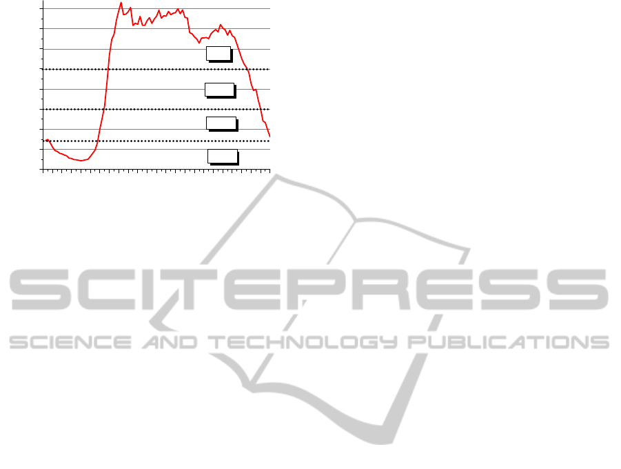
4.2 Lighting Class Reduction

Figure 2 shows the averaged daily trafﬁc intensity for

subsequent quarters as measured by induction loops

installed in a double carriageway road in the city of

Cracow, Poland (Google Map, 2015). The avg. car-

riageway width on the considered section is 9.3 m

and the avg. lamp spacing is 23.4 m. The compu-

tations were performed for the mounting height 8 m

and the LED ﬁxture BGP353 T45 DW ECO181. For

each quarter a lighting class was determined and the

corresponding LFR was established.

As speciﬁed by the standard the lighting class may

be reduced for the considered road from ME2 through

ME3b to ME4a during a day, dependently on the traf-

ﬁc intensity (see Fig.2). Obviously, we estimate en-

ergy savings in the night/twilight periods (3:30 pm to

7:15 am) only for the days of the trafﬁc measurement

(beginning of December).

Since the energy usage is calculated as the

weighted mean:

E = Σ

i∈{ME2,ME3b,ME4}

LFR

× P

× ∆t

where P

is the installation’s nominal power and ∆t

stands for an operating time for a given class, we may

easily assess the power saving ratio (α) by dividing:

α =

i∈{ME2,ME3b,ME4}

LFR

× ∆t

LFR

ME2

× [Total operating time]

For the analyzed case we obtained α = 0.73 which

means that 27% savings may be reached.

The annual mean of an operating time is assumed to be

12 h.

SMARTGREENS2015-4thInternationalConferenceonSmartCitiesandGreenICTSystems

286

00.45

01.45

02.45

03.45

04.45

05.45

06.45

07.45

08.45

09.45

10.45

11.45

12.45

13.45

14.45

15.45

16.45

17.45

18.45

19.45

20.45

21.45

22.45

23.45

5000

10000

15000

20000

25000

30000

35000

40000

Est. number of vehicles per day

Hour

ME4a

ME3b

ME2

Figure 2: Average daily trafﬁc intensity. Dotted lines sepa-

rate lighting categories corresponding to intensity size.

5 CONCLUSIONS

Large annual costs of street lighting which are ex-

pected to reach over $42 billion by 2025 encourage

to search for new methods of reducing the power us-

age. The proposed concept of lighting proﬁles allows

for combining two such approaches based on day-

light harvesting and lighting class reduction respec-

tively. This methodology is tested in two projects:

Green AGH Campus smart grid project and ISE R&D

project, basing on PhoCa software which was devel-

oped at the AGH University.

Analyzed cases and obtained results show that this

methods lead to signiﬁcant energy and cost savings.

In the presented case it was 6% energy saving by

considering ambient lighting and 23% with respect of

road class reduction.

In the future works we will focus on the impact of

an artiﬁcial ambient light which properties are signif-

icantly different than for the natural one. In particular

it is anisotropic and distance dependent.

REFERENCES

Archana, M. and Mahalahshmi, R. (2014). E – Street:

LED Powered Intelligent Street Lighting System with

Automatic Brightness Adjustment Based On Climatic

Conditions and Vehicle Movements. International

Journal of Advanced Research in Electrical, Electron-

ics and Instrumentation Engineering, 3(2):60–67.

Commission Internationale de l‘Eclairage (2010). Light-

ing of Roads for Motor and Pedestrian Trafﬁc, CIE

115:2010. Vienna: CIE.

Google Map (2015). Słowackiego Av., Cracow, PL. https://

goo.gl/maps/rlxy5. [Online; accessed 2-February-

2015].

Illuminating Engineering Society of North America

(IESNA) (2000). American National Standard Prac-

tice For Roadway Lighting, RP-8-00. New York:

IESNA.

Joshi, M., Madri, R., Sonawane, S., Gunjal, A., and Son-

awane, D. (2013). Time based intensity control for en-

ergy optimization used for street lighting. In India Ed-

ucators’ Conference (TIIEC), 2013 Texas Instruments,

pages 211–215.

Kotulski, L., Landtsheer, J. D., Penninck, S., Se¸dziwy, A.,

and Wojnicki, I. (2013). Supporting energy efﬁciency

optimization in lighting design process. Proc. of 12th

European Lighting Conference Lux Europa, Krakow,

17-19 September 2013.

Long, X., Liao, R., and Zhou, J. (2009). Development of

street lighting system-based novel high-brightness led

modules. Optoelectronics, IET, 3(1):40–46.

OSRAM (2015). Arquicity street luminaires by Arquiled

save electricity with LEDs and sensors from OSRAM

Opto Semiconductors. http://goo.gl/HpcQ4o. [On-

line; accessed 15-March-2015].

Standardization, E. C. F. (2003a). Road lighting - Part 2:

Performance requirements, EN 13201-2:2003. Ref.

No. EN 13201-2:2003 E.

Standardization, E. C. F. (2003b). Road lighting - Part 3:

Calculation of performance, EN 13201-3:2003. Ref.

No. EN 13201-3:2003 E.

Standardization, E. C. F. (2004). Road lighting - Part 1:

Selection of lighting classes, CEN/TR 13201-1. Ref.

No. CEN/TR 13201-1:2004: E.

Whitepaper by Echelon (2015). Outdoor Street Lighting.

http://goo.gl/mfpGYT. [Online; accessed 2-February-

2015].

Wikipedia (2015). Twilight duration. http://en.

wikipedia.org/wiki/Twilight#Duration. [Online; ac-

cessed 2-February-2015].

ANewApproachtoPowerConsumptionReductionofStreetLighting

287