Selective Use of Optimal Image Resolution for Depth from Multiple
Motions based on Gradient Scheme
Norio Tagawa and Shoei Koizumi
Graduate School of System Design, Tokyo Metropolitan University, 6-6 Asahigaoka, Hino, Tokyo, Japan
Keywords:
Direct Shape Recovery from Motion, Gradient Method, Random Camera Motions, FixationalEye Movements.
Abstract:
The gradient-based depth from motion method is effective for obtaining a dense depth map. However, the
accuracy of the depth map recovered only from two successive images is not so high, and hence, to increase
the depth information by tracking corresponding image points through an image sequence is often performed
by using, for example, the Kalman filter-like technique. Alternatively, multiple image pairs generated by
random small camera rotations around a reference direction can be used for gaining much information of
depth without such the tracking procedure. In the framework of this strategy, in this study, to further improve
the accuracy, we propose a selective use of the optimal image resolution. The appropriate resolution image
is required to have a linear intensity pattern which is the most important supposition for the gradient method
often used for dense depth recovery based on the theory of “shape from motion.” The performance of our
proposal is examined through numerical evaluations using artificial images.
1 INTRODUCTION
The gradient-based depth from motion methods have
been vigorously studied to recover a dense depth map
(Horn and Schunk, 1981), (Simoncelli, 1999), (Bruhn
and Weickert, 2005), (Tagawa et al., 2008), (Brox
and Malik, 2011), (Ochs and Brox, 2012). How-
ever, the accuracy of the depth map recovered from
two successive images is not enough, and hence some
methods track corresponding points in an image se-
quence to use multiple viewpoint. The accurate track-
ing is also difficult and the various techniques have
been studied, for example, based on the Kalman filter
(Paramanand and Rajagopalan, 2012) and the parti-
cle filter. We proposed a tracking method, too, which
adopts the Bayesian label assignment instead of ex-
plicit tracking (Ikeda et al., 2009). If possible, the
accurate depth recovery with no use of the tracking is
desired.
The accuracy of the gradient method hardly de-
pends on the equation error of the gradient equation.
The gradient equation is a first order approximation
of the intensity invariant constraint before and after
the relative motion between a camera and an object,
and in general the second and more higher order terms
causes the equation error. The amount of the error de-
pends on the relative relation between the size of the
image motion called an optical flow and the spatial
frequency of an image intensity pattern. This means
that the appropriate spatial frequency exists at each
pixel respectively according to the size of the opti-
cal flow. Therefore, we can select the optimal image
resolution including the effective frequency and use
it for the gradient equation. However, if the images
have little variations of the spatial frequency, the opti-
mal frequency component will not necessarily be ex-
tracted at each pixel according to the specific optical
flow determinedby the depth at that pixel and the rela-
tive camera motion. To avoid the problem, we should
analyze many intensity pairs, i.e., many optical flows
for each 3-D point on a target object.
On the other hand, the depth recovery method us-
ing random camera rotations imitating fixational eye
movements of a human’s eye ball (Martinez-Conde
et al., 2004) has been proposed (Tagawa, 2010). In
this method, since a camera is assumed to rotate ran-
domly around the reference direction with a small ro-
tation angle, the gradient method is applied simul-
taneously to a lot of image pairs without the image
point tracking. In the usual framework of the gra-
dient method, the optical flow is detected based on
the gradient equation in the first step, and next, the
depth map is recovered from the optical flow. This
two step procedure is not suitable for expanding the
gradient scheme for multiple image pairs, and the di-
rect method is adopted in (Tagawa, 2010), in which
92
Tagawa N. and Koizumi S..
Selective Use of Optimal Image Resolution for Depth from Multiple Motions based on Gradient Scheme.
DOI: 10.5220/0005462500920099
In Proceedings of the 5th International Workshop on Image Mining. Theory and Applications (IMTA-5-2015), pages 92-99
ISBN: 978-989-758-094-9
Copyright
c
 2015 SCITEPRESS (Science and Technology Publications, Lda.)

the depth map is directly recoveredwithout the optical
flow detection. In this study, we propose the selective
use of the optimal image resolution in the framework
of the method in (Tagawa, 2010)
In the following, the outline of the method in
(Tagawa, 2010) is explained in Sec. 2, and the pro-
posed method for the optimal resolution selection and
its effectiveness confirmed by numerical evaluations
are referred in Sec. 3. We show the conclusions of
this study in Sec. 4.
2 OUTLINE OF DEPTH FROM
MULTIPLE IMAGE PAIRS
2.1 Camera Motions Imitating Tremor
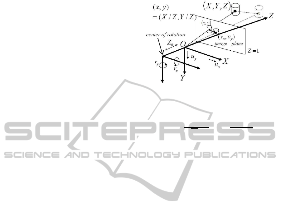
The camera coordinate system and the camera mo-
tion model imitating tremor, which is one of the fixa-
tional eye movements and is smallest one (Martinez-
Conde et al., 2004), in this study are the same as
those in (Tagawa, 2010) and are shown in Fig. 1. We
use a perspective projection system as our camera-
imaging model. A space point (X,Y,Z)
⊤
on an ob-
ject is projected to an image point ~x ≡ (x,y,1)
⊤
=
(X/Z,Y/Z,1)
⊤
.
On the analogy of a human eyeball, we can set
a camera’s rotation center at the back of a lens cen-
ter with Z
0
along an optical axis, and we assume
that there is no explicit translational motions of a
camera. This rotation with the rotational vector~r =
(r
X
,r
Y
,r
Z
)
⊤
can also be represented using the coor-
dinate origin as its rotation center with the same ro-
tational vector ~r. On the other hand, this difference
between the origin and the rotation center causes a
translational vector ~u = (u
X
,u
Y
,u
Z
)
⊤
implicitly, and
is formulated as follows:


u
X
u
Y
u
Z


=


r
X
r
Y
r
Z


×


0
0
Z
0


= Z
0


r
Y
−r
X
0


. (1)
With this system, Z
0
can be simply known before-
hand, hence an absolute depth can be recovered, al-
though a general camera motion enables us to get only
relative depth.
From Eq. 1, it can be known that r
Z
causes no
translations. Therefore, we set r
Z
= 0 and define
~r = (r
X
,r
Y
,0)
⊤
as a rotational vector like an eyeball.
~r(t) can be treated as a stochastic white Gaussian pro-
cess, in which t indicates time measured from a ref-
erence time. The fluctuation of ~r(t) at each time is
assumed to be a two-dimensional Gaussian distribu-
tion with a mean 0 and a variance σ
2
r
, where σ
2
r
is
Figure 1: Coordinate system and camera motion model
used in this study.
assumed to be known.
p(~r(t)|σ
2
r
) =
1
(
√
2πσ
r
)
2
exp

−
~r(t)
⊤
~r(t)
2σ
2
r

. (2)
In the above description, we define ~r as a rota-
tional velocity to make a theoretical analysis simple.
For small values of the actual rotation angle, Eq. 1 and
the other equations below approximate finite camera
motions.
2.2 Depth from Multiple Image Pairs
based on Gradient Method
Using the camera motion model described above and
the inverse depth d(x,y) ≡ 1/Z(x,y), the optical flow
~v ≡ [v
x
,v
y
]
⊤
is formulated as follows:
v
x
= xyr
x
−(1+ x
2
)r
y
+ yr
z
−Z
0
r
y
d ≡v
r
x
−r
y
Z
0
d,
(3)
v
y
= (1 + y
2
)r
x
−xyr
y
−xr
z
+ Z
0
r
x
d ≡v
r
y
+ r
x
Z
0
d.
(4)
In the above equations, d is an unknown variable at
each pixel, and~u and~r are unknown common param-
eters for all pixels.
At each pixel position (x, y), the gradient equation
is formulated with the partial differentials f
x
, f
y
and f
t
of the image brightness f(x, y,t) and the optical flow
as follows (Horn and Schunk, 1981):
f
t
= −f
x
v
x
− f
y
v
y
, (5)
where t denotes time. By substituting Eqs. 3 and 4
into Eq. 5, the gradient equation representing a rigid
motion constraint can be derived explicitly
f
t
= −( f
x
v
r
x
+ f
y
v
r
y
) −(−f
x
r
y
+ f
y
r
x
)Z
0
d
≡ −f
r
− f
u
d. (6)
M is the number of pairs of two successive frames
and N is the number of pixels. We assume that f
(i, j)
t
SelectiveUseofOptimalImageResolutionforDepthfromMultipleMotionsbasedonGradientScheme
93

has a Gaussian random error corresponding to the
equation error, and f
(i, j)
x
and f
(i, j)
y
have no error.
p( f
(i, j)
t
|d
(i)
,~r
( j)
,σ
2
o
) =
1
√
2πσ
o
×exp





−

f
(i, j)
t
+ f
r
(i, j)
+ f
u
(i, j)
d
(i)

2
2σ
2
o





, (7)
where i = 1,··· ,N and j = 1,··· ,M, and σ
2
o
is an un-
known variance.
Since multiple frames vibrated by irregular rota-
tions {~r
( j)
}are used for depth recovery without track-
ing of the corresponding points in the images, the re-
covered d
(i)
at each pixel takes an average value of
the neighboring region defined by vibration width in
image. Therefore, {d
(i)
} should be assumed to have
local correlation in the image. In this study, to sim-
plify the stochastic modeling of {d
(i)
}, we adopt the
following equation as the depth model.
p(
~
d|σ
2
d
) =
1
(
√
2πσ
d
)
N
exp
(
−
~
d
⊤
~
L
~
d
2σ
2
d
)
, (8)
where
~
d is a N-dimensionalvector composedof {d
(i)
}
and
~
L indicates the matrix corresponding to the 2-
dimensional Laplacian operator. By assuming this
probabilistic density, we make a recovered depth map
smooth. The use of the prior distribution of the val-
ues to be estimated is interpreted as a regularization
scheme in the signal processing viewpoint (Poggio
et al., 1985). In this study, the variance σ
2
d
is con-
trolled heuristically in consideration of smoothness of
a recovered depth map. Hereafter, we use the defini-
tion Θ ≡ {σ
2
o
,σ
2
r
}.
Based on the probabilistic models of ~r
( j)
, f
(i, j)
t
and d
(i)
defined above, we can statistically estimate
the depth map. By applying the MAP-EM algo-
rithm (Dempster et al., 1977), {
~
d, Θ} can be esti-
mated as a MAP estimator based on p(
~
d,Θ|{f
(i, j)
t
}),
which is formulated by marginalizing the joint prob-
ability p({~r
( j)
},
~
d,Θ|{f
(i, j)
t
}) with respect to {~r
( j)
},
in which the prior of Θ is formally regarded as
an uniform distribution. The concrete formula of
p(
~
d,Θ|{f
(i, j)
t
}) is shown in Eq. 15 in the AP-
PENDIX. Additionally, {~r
( j)
} can be estimated as a
MAP estimator based on p({~r
( j)
}|{f
(i, j)
t
},
ˆ
Θ,
ˆ
~
d), in
which ˆ· means a MAP estimator. The concrete for-
mula of it is also introduce in the APPENDIX by
Eq. 17. Form the formulations, the direct MAP es-
timation of
~
d is realized to be difficult, but the MAP-
EM algorithm can solve it stably through an indirect
iterative scheme each iteration of which consists of
the E-step and the M-step. In the concrete update pro-
cedure of
~
d, we use the One-Step-Late (OSL) tech-
nique (Green, 1990) to avoid complicated computa-
tion of . The details of the algorithm are shown in
(Tagawa, 2010).
3 ACCURATE RECOVERY BY
OUTLIER REDUCTION
3.1 Selection of Optimal Resolution for
Gradient Equation
The gradient equation in Eq. 5 is a linear approxima-
tion of the intensity invariant constraint before and af-
ter the relative camera motion. In general, there are
the second and more higher order terms which are
considered as the equation error included in the obser-
vation of f
t
, which is defined as a simple difference
between successive images like conventional many
methods, and cause the recovery error of the depth
map. The amount of these unwanted terms depend on
the relative relation between the spatial frequency of
the intensity pattern and the size of the optical flow at
each pixel. Therefore, in this study, we try to improve
the accuracy of the recovered depth by selecting and
using the suitable spatial frequency component and
discarding the other components as an outlying data
for each image pair.
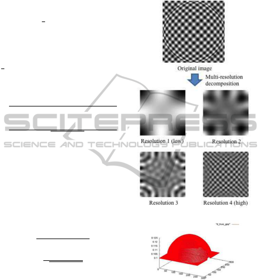
After multi-resolution decomposition shown in
Fig. 2, the proposed strategy consists of two steps.
In the first step, to detect the spatial frequency by
which drastically large amount of the equation er-
ror is observed in the gradient equation. As one
of the indices, we use the consistency of the spa-
tial gradient vectors between two successive frames
at each pixel,
~
f
(i, j)
s
≡ [ f
(i, j)
x
, f
(i, j)
y
]
⊤
and
~
f
(i, j−1)
s
≡
[ f
(i, j−1)
x
, f
(i, j−1)
y
]
⊤
. It should be noted that low resolu-
tion images are likely to generate small equation error
as compared with high resolution images but high res-
olution images can be used to recover high resolution
depth map. Hence, from low resolution to high reso-
lution at each pixel, we search the resolution in which
the directions of the spatial gradient between the suc-
cessive frames are reverse using the sign of the inner
product
~
f
(i, j)
s
⊤
~
f
(i, j−1)
s
. The image components whose
resolution is lower than the resolution in which the
sigh of
~
f
(i, j)
s
⊤
~
f
(i, j−1)
s
is negative are selected as the
candidates for the most appropriate resolution.
In the second step, the amount of the nonlinear
terms included in the observation of f
t
is estimated,
and using it the most appropriate resolution is de-
IMTA-52015-5thInternationalWorkshoponImageMining.TheoryandApplications
94

tected and is used to recover the depth at each pixel.
f
t
is exactly represented as follows:
f
t
= −f
x
v
x
− f
y
v
y
−
1
2

f
xx
v
2
x
+ f
yy
v
2
y
+ 2f
xy
v
x
v
y

+···.
(9)
If the first step is performed well, the nonlinear term
can be considered small, and in this case the second
order term in Eq. 9 can be estimated at each pixel i as
follows:
−
1
2
n
( f
(i, j)
x
− f
(i, j−1)
x
)v
(i, j)
x
+ ( f
(i, j)
y
− f
(i, j−1)
y
)v
(i, j)
y
o
.
(10)
Spontaneously, we can define two measures for esti-
mating the amount of the equation error.
J
1
=
|( f
(i, j)
x
− f
(i, j−1)
x
)v
(i, j)
x
+ ( f
(i, j)
y
− f
(i, j−1)
y
)v
(i, j)
y
|
2|f
(i, j)
x
v
(i, j)
x
+ f
(i, j)
y
v
(i, j)
y
|
,
(11)
J
2
=
|( f
(i, j)
x
− f
(i, j−1)
x
)v
(i, j)
x
+ ( f
(i, j)
y
− f
(i, j−1)
y
)v
(i, j)
y
|
2
q
f
(i, j)
x
2
+ f
(i, j)
y
2
.
(12)
J
1
measures the nonlinearity as a ratio for the amount
of the first term, which can be interpreted a signal-to-
noise ratio. We can know the merit of J
1
from Eq. 11
that J
1
can be estimated using only the direction of the
true optical flow, namely the amplitude of the optical
flow is not required to be known. J
2
measures the
nonlinearity with the dimension of the optical flow,
and this amount is proportional to the recovery error
of d.
Additionally, to estimate the higher order terms in-
cluding the second order term the following two mea-
sures can be used.
J
3
=
|f
(i, j)
t
− f
(i, j)
t0
|
|f
(i, j)
x
v
(i, j)
x
+ f
(i, j)
y
v
(i, j)
y
|
, (13)
J
4
=
|f
(i, j)
t
− f
(i, j)
t0
|
q
f
(i, j)
x
2
+ f
(i, j)
y
2
, (14)
where f
(i, j)
t0
is a true value of f
t
. For the candidate
resolutions selected in the first step, the most appro-
priate resolution for depth recovery is determined by
comparing the value of one selected from J
k
(k =
1,2, 3,4). It is noted that the exact values of these
measures cannot be computed, since these include the
variables to be determined. Therefore, only those es-
timates are provided.
3.2 Numerical Evaluation
To confirm the effectiveness of the proposed method,
and especially compare the efficiency of J
k
(k =
Figure 2: Example of multi-resolution decomposition.
Figure 3: True depth map used for evaluation.
1,2, 3,4), we conducted numerical evaluations using
artificial images. Figure 3 shows the true inverse
depth map for evaluation. The vertical axis indi-
cates the inverse depth d using the focal length as a
unit, and the horizontal axes represent the pixel posi-
tion in the image plane. The reference image gen-
erated by a computer graphics technique is shown
in Fig. 2. The images viewed with random cam-
era motions are generated using the reference image,
the true depth map and the random camera rotations
SelectiveUseofOptimalImageResolutionforDepthfromMultipleMotionsbasedonGradientScheme
95

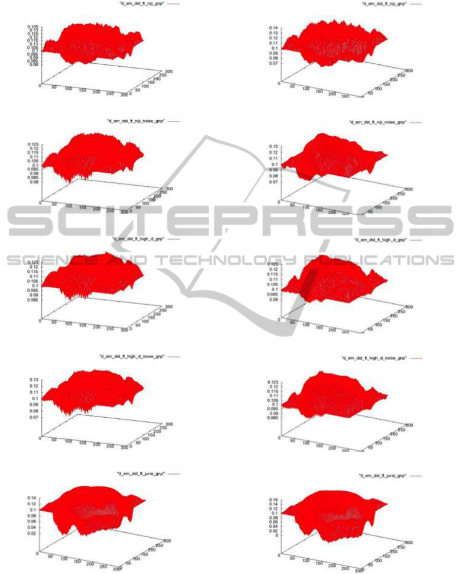
(a)
(b)
(c)
(d)
(e)
Figure 4: Recovered depth map with σ
2
r
= 0.006
2
: appro-
priate resolution is selected using (a) J
1
, (b) J
2
, (c) J
3
, (d)
J
4
, and (e) result by conventional method.
(a)
(b)
(c)
(d)
(e)
Figure 5: Recovered depth map with σ
2
r
= 0.008
2
: appro-
priate resolution is selected using (a) J
1
, (b) J
2
, (c) J
3
, (d)
J
4
, and (e) result by conventional method.
IMTA-52015-5thInternationalWorkshoponImageMining.TheoryandApplications
96

sampled as a Gaussian independent random variable
defined in Eq. 2. The image size adopted in these
evaluations is 256×256 pixels, which corresponds to
−0.5 ≤ x,y ≤ 0.5 measured using the focal length as
a unit. All images were decomposed into four res-
olution layers shown in Fig. 2. We recovered the
depth map from a image set consisting of 100 im-
ages each having random movements. Image pairs
consist of each image and the reference image were
used to compute f
x
, f
y
and f
t
in the gradient equa-
tion. The most appropriate resolution was determined
by the method explained in the above section at each
pixel in each image pair, and was used as an observa-
tion for the MAP-EM algorithm. A plane Z = 9 was
used as an initial value of the depth map. The param-
eter σ
2
d
determining the degree of smoothness of the
recovered depth was fixed as σ
2
d
= 1.0×10
−4
, and the
accuracy of the recovereddepth map was evaluated by
varying σ
2
r
determining the amplitude of the random
camera rotations.
In this evaluation, firstly we use the true value of
the optical flow for computing J
k
(k = 1, 2,3,4) to
confirm the essential effectiveness of the selective use
of the spatial frequency. Figure 4 shows the recovered
inverse depth map for σ
2
r
= 0.006
2
. Likewise, Fig. 5
shows the results for σ
2
r
= 0.008
2
, i.e. the results for
the large motions compared with Fig. 4. In the fig-
ures, the conventional method (Tagawa, 2010) indi-
cates that the image intensity is used as is, namely se-
lective use of the optimal resolution is not performed.
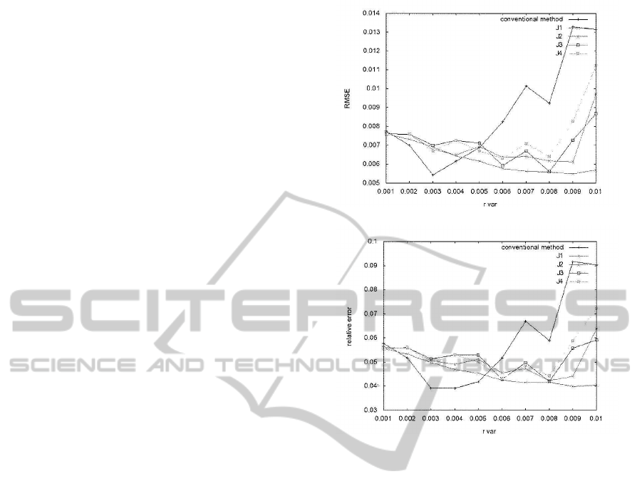
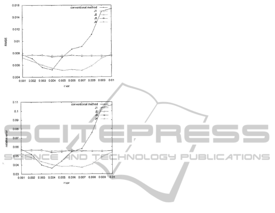
Figure 6 represents the relation between the depth re-
covery error and the amplitude of the random camera
rotations. From both of the root mean square error
(RMSE) and the relative error, we can confirm that
the proposed outlier reduction is in effect especially
for the large camera rotations. For relatively small
camera rotations, the proposed all measures can be
used to improve the accuracy of In the four measures,
J
1
shows good performance regardless of size of the
camera motion.
Successively, we evaluate the actual case in which
the true optical flow is unknown. At each pixel in each
image pair, the minimum least square solution of the
optical flow is derived using the candidate resolutions
selected by the first step in the proposed method, and
is used for compute J
k
(k = 1,2, 3,4). The relation
between the depth recovery error and the amplitude of
the random camera rotations are sown in Fig. 7. As a
result, the performance of J
1
was still in effect, which
is expected to be caused by the fact that J
1
depends
only on the direction of the optical flow.
(a)
(b)
Figure 6: Recovery error vs. amplitude of camera rotation
evaluated using true values of optical flow: (a) RMSEs, (b)
relative errors.
4 CONCLUSIONS
In this study, we examine the method to improve the
accuracy of the depth recovery based on the rela-
tive camera motions. We focused on the linear ap-
proximation error of the gradient equation, and pro-
posed the selective use of the optimal image reso-
lution. We defined different four measures to esti-
mate the approximation error, and the effectiveness
was confirmed by integrating the proposed selection
method into the conventional depth recovery method
using random camera rotations. In the future, real im-
age experiments have to be carried out to indicate the
actual performance of our method.
We are now proceeding with the further examina-
tion to improve the accuracy of the recovered depth,
in which we adopt Eq. 10 for the representation of the
second order term included in the observed f
t
for the
resolution selected by the measure J
1
. By this repre-
sentation, the gradient equation corresponding to the
second order approximation of the intensity invari-
ant constraint can be formulated as a linear equation
SelectiveUseofOptimalImageResolutionforDepthfromMultipleMotionsbasedonGradientScheme
97

(a)
(b)
Figure 7: Recovery error vs. amplitude of camera rotation
using estimates of optical flow: (a) RMSEs, (b) relative er-
rors.
about an optical flow, which is easy to be handled. It
is noted that this formulation is nothing but redefin-
ing a spatial gradient of intensity patterns using the
intensity of two sucsessive images.
In the framework using random camera rotations,
the integral-formed method based on motion blur has
also proposed. This method is effective for the large
image motions compared with the image intensity
patterns, and hence, it can be used for the case in
which the differential-formed method in this study
is not suitable (Tagawa et al., 2012), (Tagawa et al.,
2013). Unification of both schemes is a future prob-
lem, too.
REFERENCES
Brox, T. and Malik, J. (2011). Large displacement opti-
cal flow: descriptor matching in vartional motion es-
timation. IEEE Trans. Pattern Anal. Machine Intell.,
33(3):500–513.
Bruhn, A. and Weickert, J. (2005). Locas/kanade meets
horn/schunk: combining local and global optic flow
methods. Int. J. Comput. Vision, 61(3):211–231.
Dempster, A. P., Laird, N. M., and Rubin, D. B. (1977).
Maximum likelihood from incomplete data. J. Roy.
Statist. Soc. B, 39:1–38.
Green, P. J. (1990). On use of the em algorithm for pe-
nalized likelihood estimation. J. Roy. Statist. Soc. B,
52:443–452.
Horn, B. P. and Schunk, B. (1981). Determining optical
flow. Artif. Intell., 17:185–203.
Ikeda, M., Okubo, K., and Tagawa, N. (2009). Implicit
tracking of multiple objects based on bayesian region
label assignment. In proc. VISAPP2009, pages 503–
506.
Martinez-Conde, S., Macknik, S. L., and Hubel, D. (2004).
The role of fixational eye movements in visual percep-
tion. Nature Reviews, 5:229–240.
Ochs, P. and Brox, T. (2012). Higher order motion models
and spectral clustering. In proc. CVPR2012, pages
614–621.
Paramanand, C. and Rajagopalan, A. N.(2012). Depth from
motion and optical blur with unscented kalman filter.
IEEE Trans. Image Processing, 21(5):2798–2811.
Poggio, T., Torre, V., and Koch, C. (1985). Computational
vision and regularization theory. Nature, 317:314–
319.
Simoncelli, E. P. (1999). Bayesian multi-scale differential
optical flow. In Handbook of Computer Vision and
Applications, pages 397–422. Academic Press.
Tagawa, N. (2010). Depth perception model based on fix-
ational eye movements using byesian statistical infer-
ence. In proc. ICPR2010, pages 1662–1665.
Tagawa, N., Iida, Y., and Okubo, K. (2012). Depth per-
ception model exploiting blurring caused by random
small camera motions. In proc. Int. Conf. on Com-
puter Vision, Theory and Applications, pages 329–
334.
Tagawa, N., Kawaguchi, J., Naganuma, S., and Okubo, K.
(2008). Direct 3-d shape recovery from image se-
quence based on multi-scale bayesian network. In
proc. ICPR08, page CD.
Tagawa, N., Koizumi, S., and Okubo, K. (2013). Direct
depth recovery from motion blur caused by random
camera rotations imitating fixational eye movements.
In proc. Int. Conf. on Computer Vision, Theory and
Applications, pages 177–186.
APPENDIX
The posterior distribution of
~
d and Θ is derived using
the Bayes’ theorem and the uniform prior probability
p(Θ) = Const. as follows:
IMTA-52015-5thInternationalWorkshoponImageMining.TheoryandApplications
98

p(
~
d,Θ|{f
(i, j)
t
}) =
p(
~
d, Θ,{f
(i, j)
t
})
p({f
(i, j)
t
}
∝
Z
···
Z
p({f
(i, j)
t
},{~r
( j)
},
~
d,Θ)d{~r
( j)
}
=
Z
···
Z
p({f
(i, j)
t
}|{~r
( j)
},
~
d,σ
2
o
)p({~r
( j)
}|σ
2
r
)p(
~
d|σ
2
d
)
×p(Θ)d{~r
( j)
}
∝
Z
···
Z
N
∏
i=1
M
∏
j=1
p( f
(i, j)
t
|d
(i)
,~r
( j)
,σ
2
o
)
M
∏
j=1
p(~r
( j)
|σ
2
r
)
×p(
~
d|σ
2
d
)d{~r
( j)
}
=
1
(2π)
N(M+1)/2+M
σ
MN
o
σ
2M
r
σ
N
d
×
Z
···
Z
exp





−
∑
N
i
∑
M
j

f
(i, j)
t
+ ~w
(i, j)⊤
~r
( j)

2
2σ
2
o
−
∑
M
j=1
~r
( j)⊤
~r
( j)
2σ
2
r
)
d{~r
( j)
}exp
(
−
~
d
⊤
~
L
~
d
2σ
2
d
)
, (15)
~w
(i, j)
≡



f
(i, j)
x
x
(i)
y
(i)
+ f
(i, j)
y
(1+ y
(i)
2
)
−f
(i, j)
x
(1+ x
(i)
2
) − f
(i, j)
y
x
(i)
y
(i)
f
(i, j)
x
y
(i)
− f
(i, j)
y
x
(i)



+Z
0
d
(i)



f
(i, j)
y
−f
(i, j)
x
0



. (16)
The posterior distribution of {~r
( j)
} is also derived
as follows:
p({~r
( j)
}|{f
(i, j)
t
},Θ,
~
d) =
p({~r
( j)
},{f
(i, j)
t
}|Θ,
~
d)
p({f
(i, j)
t
}|Θ,
~
d)
∝ p({f
(i, j)
t
}|{~r
( j)
},
~
d,σ
2
o
)p({~r
( j)
}|σ
2
r
)
=
1
q
(2π)
2M
∏
M
i
det
~
V
( j)
r
×exp
(
−
1
2
M
∑
j=1

~r
( j)
−~r
( j)
m

⊤
~
V
( j)
r
−1

~r
( j)
−~r
( j)
m

)
,
(17)
~r
( j)
m
= −
1
σ
2
o
~
V
( j)
r
N
∑
i=1
f
(i, j)
t
~w
(i, j)
, (18)
~
V
( j)
r
=
1
σ
2
o
N
∑
i=1
~w
(i, j)
~w
(i, j)⊤
+
1
σ
2
r
~
I
!
−1
. (19)
SelectiveUseofOptimalImageResolutionforDepthfromMultipleMotionsbasedonGradientScheme
99