An Explanation of the Physical Origin of the Extra-ordinary Angular

Tolerance of Cavity Resonator Integrated Grating Filters

Nadège Rassem, Anne-Laure Fehrembach and Evgeni Popov

Université d'Aix-Marseille, CNRS, Centrale Marseille, Institut Fresnel, Marseille, France

Keywords: Gratings, Subwavelength Structures, Bragg Reflectors, Eigenvalues, Resonance Domain.

Abstract: Cavity – resonator - integrated guided - mode resonance filters (CRIGFs) are promising structures that afford

a very fine spectral width less than 1 nm. We study another structure to compare compare it to CRIGF. The

angular acceptance of CRIGF is an order of magnitude greater than in classical gratings, even with complex

pattern. To identify the phenomenon responsible for the extraordinary large angular acceptance of CRIGF,

we study the dispersion curve of the mode excited in the CRIGF.

1 INTRODUCTION

With the increase of applications requiring spectral

filtering, free space optical filters are the focus of

several studies.

Fabry-Perot multilayer filters are the most widely

used free space filters but show limits for narrow band

filtering. To get a narrow spectral width with this type

of filters, one needs a large number of layers thus

increasing the size of the component which becomes

unstable over time and with temperature.

Resonant grating filters are a very promising

alternative relative to conventional multilayer filters.

The resonant grating filter is composed of a stack of

several dielectric layers on top of which a periodic

nanostructure is engraved. The multilayer stack plays

the role of a planar waveguide and the engraved

structure allows to couple and decouple one

eigenmode of the structure to the incident wave

through one diffraction order of the grating. When

the component is illuminated, a resonance peak

occurs in the reflectivity or transmittivity spectrum.

The characteristics of the peak, namely the centering

wavelength and width, are mainly governed by the

grating parameters. Those resonant grating structures

are commonly called GMRF (Guided-mode

Resonance Filters) and are known to have a very

small angular tolerance. However they have a high

quality factor and a very high rate of rejection.

The small angular tolerance is observed especially

when the GMRF is illuminated under oblique

incidence. That is to say when one single mode is

excited through one diffraction order, usually the first

order. In this configuration, it is possible to show

(Evenor et al., 2012).

The spectral and angular width depends on the

same parameters of the grating, namely the height h

of the grating and its 1st Fourier coefficient. A small

angular tolerance leads up to the degradation of the

rate of rejection and to the spreading of the spectrum

when the grating is illuminated with a beam with a

large divergence. But if our grating is illuminated

under normal incidence, two counter propagating

modes are excited. In this configuration, the angular

width depends on the 2nd Fourier coefficient while

the spectral width depends on the first coefficient as

shown in. (Evenor et al., 2012). Resonant grating

filters with complex basic pattern have been proposed

(Fehrembach et al., 2010), leading to an angular width

of 0.5° at 1550nm for a bandwidth of 0.28nm. Yet,

these record performance may be still insufficient for

applications where the component have to be

illuminated with a focused beam. In this optic another

structure called CRIGF was introduced (X. Buet et

al., 2012) and (K. Kintaka et al., 2012). It consists of

a GMRF and a pair of distributed Bragg reflectors

(DBRs) constructing a waveguide cavity resonator.

We inserted a phase section between each DBR and

the GMRF to optimize the reflectivity of the CRIGF.



Rassem N., Fehrembach A. and Popov E..

An Explanation of the Physical Origin of the Extra-ordinary Angular Tolerance of Cavity Resonator Integrated Grating Filters.

 2015 SCITEPRESS (Science and Technology Publications, Lda.)

2 OBJECTIVES AND

COMPARISION OF THE TWO

STRUCTURES

The objective of our research is to improve the

performances of resonant gratings. To begin, we

compare two structures. The first component is

periodic and is called “doubly periodic” structure

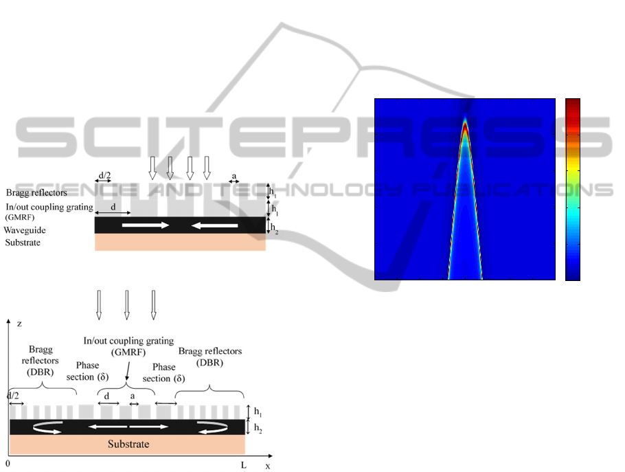
(Figure 1). It is composed with a coupling grating

(GMRF) and a Bragg grating with half filling factor

and a period two times smaller than the GMRF

grating. The two gratings are located one above the

other. The second structure (Figure 2), called CRIGF

(Cavity - Resonator -Integrated guided -mode-

resonance filters), is non-periodic it is composed with

one GMRF section and two Bragg reflector sections.

The GMRF period is d and the DBR periods is d/2.

The phase section is δ.



Figure 1: “doubly periodic" structure.

Figure 2: CRIGF structure.

The GMRF and the Bragg sections have both a

groove width a = 100 nm and depth h

= 120 nm. The

guiding layer thickness is h

= 165 nm. The indexes

of the materials are 1.46 for the gratings and 1.97 for

the guiding layer. The superstrate is air with index 1.0

(the same for the grating grooves) and the substrate is

silica, with index 1.46. The period of the central

section is d = 532 nm. The GMRF and Bragg

reflectors included in the CRIGF have the same

parameters than the “doubly periodic structure, and

the phase section of the CRIGF is δ = 1.05d. The

CRIGF is composed with 21 periods of GMRF and

200 periods.

Our aim is to compare the dispersion relations of

the periodic and the non-periodic structures.

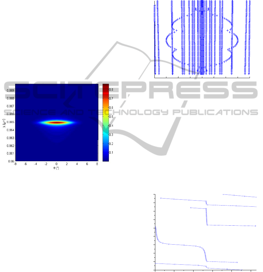
We plot on figure 3 the reflectivity versus the

wavelength λ and the polar angle of incidence θ. The

map shows a forbidden band, as it is well known for

infinite resonant gratings. The reflectivity map is

calculated for a planar incident wave. When a

Gaussian beam is used, other calculations, not plotted

here, show that the maximum of the reflectivity at

resonance decreases with the size of the beam at waist

when the beam divergence becomes too wide as

compared to the angular tolerance of the component

.



Figure 3: reflectivity of the "doubly periodic" with respect

to the angle of incidence and wavelength, showing a

forbidden band.

When we plot the reflectivity versus the

wavelength λ and the polar angle of incidence θ for

the CRIGF (figure 4), we observe a spot where the

reflectivity is maximum. The spot is centered at λ =

864.9 nm and normal incidence. The incident beam is

a Gaussian beam with a radius at waist of 5.2 µm, for

which the maximum reflectivity at resonance is

maximum (calculations not shown here).

This map is very different from that of the infinite

grating plotted in figure 3. When the angle of

incidence increases (in absolute value), or the

wavelength moves away from 864.9 nm, the reflected

energy decreases: the resonance degrades. This

device has a wide angular acceptance, from -2° to 2°,

together with a thin spectral width. The results of the

calculations presented here were obtained using a

home-made numerical code based on the Fourier

Modal Method, also known as Rigorous Coupled

Wave Analysis (RCWA), improved by using the

more rapidly converging rules of factorization of



(°)

wavelength (



-8 -6 -4 -2 0 2 4 6 8

0.86

0.862

0.864

0.866

0.868

0.87

0.2

0.4

0.6

0.8

AnExplanationofthePhysicalOriginoftheExtra-ordinaryAngularToleranceofCavityResonatorIntegratedGrating

Filters

product of discontinuous functions enounced at (Li,

1997). The number of Fourier harmonics is truncated

to from -700 to 700. To model a CRIGF with our

RCWA code dedicated to model periodic structures,

we use the so-called ”super-cell” method, which

consists in considering the CRIGF as the basic pattern

of a grating. For the modeling to be valid, it is

necessary to isolate each basic cell from its neighbors.

For this reason, the opportunity to add an absorbing

layer between each basic cell is implemented. The

absorbing layer consists of n

slices

slices of

homogeneous layers with a total thickness L

ABS

and

are characterized by an optical index n varying as n(x)

= n(x0) + i[(x − x0)/L

ABS

]

, where x

is the x-starting

position of the absorbing layer. The absorbing layer

can be added inside the grating region, and waveguide

region.



Figure 4: R (θ, λ) map of the CRIGF.

3 EIGENVALUES

CALCULATION

To understand more the phenomenon presented on

figure 4, we studied the behavior of the complex

propagation constant of the excited eigenmode with

respect to the angle of incidence, that is to say the

dispersion relation. We employed the method

described in ref. (Q. Cao et al., 2002). It consists in

calculating the T-matrix of the structure from one

edge to the other (from x=0 to x=L, see figure 2) The

complex propagation constant g of the eigenmodes

are related to the eigenvalues  of the T matrix trough

the relation:



= exp(i



L





L being the total length of the structure. For this

calculation, the structure is repeated periodically

along the z-direction, and we include absorbing layers

between two adjacent structures.This configuration

reduces the period of the problem considered for the

numerical calculation and thus the truncation order of

the Fourier series.



Figure 5: Imaginary parts of the propagation constants of

the eigenmodes of the CRIGF with respect to the

wavelength.

We plot in figure 5 the imaginary part of the

propagation constants  with respect to the

wavelength. We can see many different eigenmodes

with imaginary parts that depend quasi linearly on the

wavelength and correspond to quasi-plane waves.

Among these values, one eigenmode has a different

behavior, showing an imaginary part that draws three

major foils as a function of the wavelength. We

identified the real part of the propagation constant of

this different eigenmode. It is plotted on figure 6.



Figure 6: Real part of the propagation constant of the

interesting eigenmode with respect to the wavelength.

This real part is characterized by a flat portion that

appears around 864.9 nm, which corresponds to the

center wavelength of the peak observed in Figure 4.

-0.1 -0.075 -0.05 -0.025 0 0.025 0.05 0.075 0.1

0.86

0.865

0.87

0.875

imag (



) (



-1

)

wavelength (



0.00 0.01 0.02 0.03 0.04 0.05

0.858

0.860

0.862

0.864

0.866

0.868

0.870

0.872

0.874

0.876

wavelength (m)

real() (m

-1

)

PHOTOPTICS2015-DoctoralConsortium

We note that from eq. 1, the real part of the

eigenvalues is defined with an indetermination of 2

/ L = 0.0529 µm-1, L being the total length of the

structure (L = 118.6892 µm).

Bellow, we study the evolution of the dispersion

relations (the real and the imaginary part of ) when

introducing different strength of the Bragg reflectors,

by varying the number of grooves of the Bragg

grating. The central grating length is fixed constant,

so that when varying the Bragg grating length, the

length L

of the whole structure with varies.



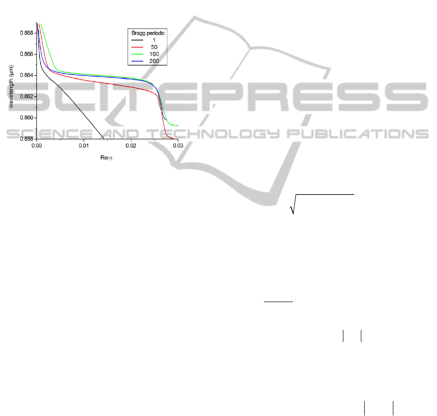
Figure 7: Evolution of the real part when varying the period

of Bragg.

We present on fig. 7 the evolution of the “good”

eigenvalues when the number of the Bragg grating

periods increases from 1 to 200. As far as the values

of real () are determined within integer times

2 / L

, in order to avoid the change in this

ambiguity, we plot the real part of  L

/ L with

respect to the wavelength, where the total

normalization length L = L

200

= 118.6892 µm is kept

fixed. We observe that the shape of the real part

changes gradually with the DBR groove numbers,

starting from the single-grating curve (calculated,

without Bragg grating, but not shown here) towards

the curve given in Figure 7. An increasingly flatter

region is formed in the wavelength interval 0.863-

0.865 µm.

In the following, we present an approached theory

derived from the coupled-mode theory which allow to

identify the physical origin of the extra-ordinary

flattening of the dispersion curve.

Let us consider a grating waveguide, invariant in

the y direction that supports leaky modes propagating

in the x direction, with the leakage

out



due to the

radiation into a propagating diffraction orders in the

substrate and the superstrate. The vector field

components of the mode

F(x, z)

can be factorized in

the form:

ik x

F(x, z) f (z)e

(2)

The propagation constant k

is real without

grating for waveguides made of lossless materials.

For a grating waveguide, the radiation losses enter in

the mode propagation constant along x and increase

its imaginary part:

ggouta.l.

kRe(k)i( )



 

(3)

with

a.l.



staying for the absorption losses, if any.

In addition to the leakage, the mode propagation

constant and field map can be modified by the

interaction between counter-propagating modes. The

classical coupled-mode theory shows that this

coupling modifies the propagation constant and forms

a forbidden gap in its dispersion map; the

modification resulting in a formation of two hybrid

modes having two slightly different propagation

constants (4):













(4)

with







(5)



is the coupling strength between the two

counter-propagating modes and is proportional to the

overlap mode integral in transverse direction. In

particular, if the interaction involves the same

counter-propagating modes and is due to the grating

that extends from 0 to h in z-direction, then

2T 2

202

k F n (x, z) f (z) dz

















(6)

and

Fn(x,z)









stays for the m-th Fourier

transform, along x, of the square of the refractive

index function of the grating.

The spectral region in which

Kk

forbidden (band gap) in the sense that the imaginary

part of the propagation constant increases due to the

backward scattering. At its boundaries, the real part



has the weakest dependence on the incident

vector component, parallel to the surface and thus the

angular tolerances of the filter response are less tight.

AnExplanationofthePhysicalOriginoftheExtra-ordinaryAngularToleranceofCavityResonatorIntegratedGrating

Filters

Let us consider the CRIGF. To calculate his

transmission matrix T

total

, we need to express the

transmission matrix of each Bragg grating, the

transmission matrix of the GMRF (middle grating)

and the transmission matrix at each interface

Bragg/GMRF. We consider that we are at the

boundary of the forbidden gap, so we have to take into

account four modes with the propagation constants

, –k

, +k

–

, –k

–

inside each region (Bragg grating

and GMRF)

(N. Rassem et al.).

We define for the Bragg grating and the GMR

respectively the transmission matrix T

and T

are expressed respectively as functions

of ±k

, ±k

At the interfaces between the Bragg grating and

GMRF, the interaction between the modes can be

expressed through four overlap integrals (see ref. 5

for the full expressions): R

for k

and k

, R

for

and k

, R

for k

and k

, and R

for k

and

We define an 8 x 8 transmission matrix R that

contains the overlap integrals.









0







0







0







0







(7)

The total transmission matrix is the product of

the transmission matrices in the Bragg gratings T

and the matrix containing the propagation in the

middle grating T

plus the interaction on the

interfaces between the different gratings (R matrix):

total B G B

TTRTRT

(8)

In order to illustrate the influence of the mode

interaction at the interface between the different

gratings, in what follows we make several reasonable

assumptions:

(1) Symmetrizing the problem by assuming that:

RRR

 

 



(9)

We shall take these coefficients as real (

1,2

RRe

)

(2) Neglecting the radiation losses due to the

transition effects on the interfaces between the

gratings, and higher mode interactions. For this aim

we consider the relation:

(10)

(3) Last, we assume that the Bragg gratings act

as if localized on the interfaces x = 0 and L

through the overlap integrals in R, i.e.,

considering the eigenvalues of

MRTR

instead of T

total

To begin, we plot on figure 8 the evolution of the

real part of the propagation constant with respect to

the wavelength for several values of R

-. We observe

a behavior that is similar to that observed for the

propagation constants calculated numerically (see

figure 7). From these curves, we can conclude that the

Bragg grating reflection plays a decisive role in the

formation of the flat part in the dispersion curve, the

stronger the coupling, the flatter the curve.

0.860

0.862

0.864

0.866

0.868

0.870

0.000 0.005 0.010 0.015 0.020 0.025 0.030

+ -

Re

wavelength (µm)

0.3

0.5

0.6

0.707



Figure 8: Evolution of the real part of the propagation

constant for varying strength of coupling between the

modes.

4 CONCLUSIONS

To sum up, we presented a study aiming at identifying

the physical origin of the extra-ordinary flattening of

the dispersion curve of CRIGF. We showed, both

from a numerical study and from an approached

model based on the coupled modes theory, that the

dispersion curve flattening increases with the

reflection on the Bragg grating. Moreover, the semi-

analytical model allows us to attribute this extra-

ordinary flattening of the dispersion curve to the

coupling between modes that does not occur in

infinite gratings. As it is well-known from the two-

waves coupled mode theory, the interaction between

two counter-propagative modes leads to a creation of

two hybrid modes, one with a larger (k

) and the other

with a smaller (k

–

) constant of propagation.

The Bragg grating cavity resonator that contains

the central GMRF grating can leads to a well-known

reflection of the mode “k

” into the mode “–k

” (and

similarly for k

–

), but also can provide an additional

coupling between the hybrid modes (“k

” into “–k

–

”)

that does not exist without the Bragg grating box. We

RR1

PHOTOPTICS2015-DoctoralConsortium

have shown that the strength of this additional

coupling (proportional to overlapping integral R

–+

) is

directly responsible for the flattening of the

dispersion curve of the mode of the entire system. In

particular, when the two types of coupling have

similar strengths, one observes an extraordinary

flattening of the dispersion curve of CRIGF devices.

In order to better understand how to improve the

performance of this component (CRIGF), we plan to

study the influence of each parameter of the structure.

REFERENCES

Evenor, I.; Grinvald, E.; Lenz, F. & Levit, S. Analysis of

light scattering off photonic crystal slabs in terms of

Feshbach resonances Eur. Phys. J. D., 2012, 66, 231-

239.

Fehrembach, A.-L.; Lemarchand, F.; Talneau, A. &

Sentenac, A. High Q polarization independent guided-

mode resonance filter with “doubly periodic” etched

Ta2O5 bidimensional grating I.E.E.E. J. Light. Tech.,

2010, 28, 2037-2044.

Q. Cao, Ph. Lalanne, and J.-P. Hugonin, “Stable and

efficient Bloch-mode computational method for one-

dimensional grating waveguides,” J. Opt. Soc. Am. 19,

335-338 (2002).

P. Paddon, and J. F. Young, “Two-dimensional vector-

coupled-mode theory for textured planar waveguides,”

Phys. Rev. B, 61, 2090 (2000).

N. Rassem, A.-L. Fehrembach, E. Popov “Waveguide

mode-in-the box with extra flat dispersion curve”,

submitted JOSAA.

Li, L. “New formulation of the Fourier modal method for

crossed surface-relief gratings” J. Opt. Soc. Am. A,

1997, 14, 2758-2767.

X. Buet, E. Daran, D. Belharet, F. Lozes-Dupuy, A.

Monmayrant and O. Gauthier-Lafaye. “High angular

tolerance and reflectivity with narrow bandwidth

cavity-resonator-integrated guided-mode resonance

filter”. Optics Express, 20:9322-9327, 2012.

K. Kintaka, T. Majima, J. Inoue, K. Hatanaka, J. Nishii and

S. Ura. “Cavity-resonator-integrated guided-mode

resonance filter for aperture miniaturization”. Optics

Express, 20:1444-1449, 2012.

AnExplanationofthePhysicalOriginoftheExtra-ordinaryAngularToleranceofCavityResonatorIntegratedGrating

Filters