On the Influence of Superpixel Methods for Image Parsing
Johann Strassburg, Rene Grzeszick, Leonard Rothacker and Gernot A. Fink
Department of Computer Science, TU Dortmund, Dortmund, Germany
Keywords:
Image Parsing, Superparsing, Segmentation, Superpixels.
Abstract:
Image parsing describes a very fine grained analysis of natural scene images, where each pixel is assigned
a label describing the object or part of the scene it belongs to. This analysis is a keystone to a wide range
of applications that could benefit from detailed scene understanding, such as keyword based image search,
sentence based image or video descriptions and even autonomous cars or robots. State-of-the art approaches
in image parsing are data-driven and allow for recognizing arbitrary categories based on a knowledge transfer
from similar images. As transferring labels on pixel level is tedious and noisy, more recent approaches build
on the idea of segmenting a scene and transferring the information based on regions. For creating these regions
the most popular approaches rely on over-segmenting the scene into superpixels. In this paper the influence of
different superpixel methods will be evaluated within the well known Superparsing framework. Furthermore, a
new method that computes a superpixel-like over-segmentation of an image is presented that computes regions
based on edge-avoiding wavelets. The evaluation on the SIFT Flow and Barcelona dataset will show that the
choice of the superpixel method is crucial for the performance of image parsing.
1 INTRODUCTION
The analysis of images is an important task for a wide
range of applications from image search to the analy-
sis of the surroundings in cars or robots. A very fine
grained analysis is a full scene labeling at pixel level,
which is also known as scene or image parsing. The
goal is to label every pixel in the image with a mean-
ingful category such as the object that is represented
at this pixel of the scene. This is a more detailed anal-
ysis than the results that are obtained by bounding
box object detectors. An example of image parsing
is shown in Fig. 1.
There are many approaches to image parsing, the
most well known ones being (Liu et al., 2011), (Tighe
and Lazebnik, 2013b) and (Farabet et al., 2013).
These approaches are data-driven and allow for rec-
ognizing arbitrary categories based on a knowledge
transfer from similar images. For a given query im-
age the most similar images are retrieved from an an-
notated dataset. Then local similarities are used in
order to transfer the information from the retrieval set
onto the query image.
In (Liu et al., 2011) the label transfer method is
based on the SIFT Flow. GIST & Bag-of-Features
representations are used as global features in order to
retrieve similar images for a given query image. Then
Query-Image
Image
Parsing
Labeled image
Sky
Mountain
Snow
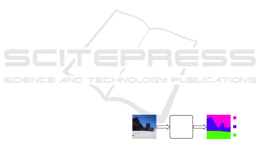
Figure 1: The idea of an image parsing system is to produce
a pixel based labeling of a scene. Here, the different regions
of the image are labeled as sky, mountain & snow.
for each pixel a SIFT descriptor is computed. The de-
scriptors from the query image are matched with the
ones of the images in the retrieval set using an objec-
tive function similar to the optical flow. Here, dense
sampling is not applied to a time series, but to a set of
images using SIFT descriptors, henceforth it is called
SIFT Flow. The retrieval set is then re-ranked using
the overall minimum flow energy and a final set of
similar images is retrieved. The correspondences be-
tween the descriptors are then used for transferring
the labels to the query image. The main disadvan-
tage of this method is the computational complexity
of computing the flow between the query image and
all images in the retrieval set. Also the dense grid that
is used for a per-pixel flow tends to be quite noisy,
creating several very small labeled regions, and is not
intuitive considering that a scene usually consists of a
set of objects.
Therefore, the more recent approaches build on
518
Strassburg J., Grzeszick R., Rothacker L. and Fink G..
On the Influence of Superpixel Methods for Image Parsing.
DOI: 10.5220/0005355705180527
In Proceedings of the 10th International Conference on Computer Vision Theory and Applications (VISAPP-2015), pages 518-527
ISBN: 978-989-758-090-1
Copyright
c
 2015 SCITEPRESS (Science and Technology Publications, Lda.)

the idea of segmenting a scene and transferring the
information based on regions. Such an approach is
presented in (Tighe and Lazebnik, 2013b), the so-
called Superparsing. The main idea can be described
in three steps. First, a set of global image features,
GIST, Bag-of-Features & a color histogram are com-
puted. Then, for a given query image the most similar
images are retrieved from an annotated dataset. Sec-
ond, the query image and the retrieval set are over-
segmented, each segment creating a set of pixels that
contains some context information, so-called super-
pixels. Each superpixel is also described by a set of
features that cover shape, location, texture, color and
appearance information. The complete set of global
& local features is described in (Tighe and Lazebnik,
2013b). Third, for each superpixel in the query image
the most similar superpixels from the retrieval set are
used in order to obtain a label.
The approach has been extended by contextual in-
ference, cf. (Tighe and Lazebnik, 2013b). An addi-
tional classifier for geometric classes (horizontal, ver-
tical, sky) is evaluated and the semantic labels for the
regions are compared to their geometric counterpart.
For example, a street is a horizontal entity and a build-
ing a vertical one. Furthermore, the neighboring su-
perpixels are taken into account, for example, a car is
unlikely to be surrounded by water or the sky. Both
conditions are integrated into a conditional random
field and used for re-weighting the classwise proba-
bilities for the semantic class labels. In (Tighe and
Lazebnik, 2013a) an extension has been proposed that
combines the superparsing approach with the output
of different per object detectors in order to improve
the results for a given set of categories.
In (Farabet et al., 2013) another region-based ap-
proach has been proposed. Instead of extracting de-
signed local image descriptors, like SIFT or HOG, a
multi-scale convolutional network is integrated into
the image parsing. The input image is transformed
with a Laplacian pyramid and a convolutional net-
work is applied to the transformed images in or-
der to compute feature maps. Again instead of a
pixel-wise evaluation of these feature maps a set
of regions is evaluated that is created by either an
over-segmentation or a multi-scale approach creating
coarse and fine sets of regions using the same over-
segmentation algorithm.
These region-based scene representations are also
very similar to the coarser analysis that is performed
in the automotive industry. Here, a column based ap-
proach and depth differences in the 3D space are used
for creating the regions, the so-called stixels (Badino
et al., 2009). Natural scenes are then labeled based on
these stixels which allows for detecting a set of rele-
vant objects, like cars, persons or buildings.
Even though several extensions have been pro-
posed, a crucial part of these state-of-the-art meth-
ods is the underlying segmentation algorithm that
computes the superpixels. All region-based ap-
proaches are based on the segmentation algorithm
from (Felzenszwalb and Huttenlocher, 2004) in order
to create an over-segmentation. In this paper the in-
fluence of different superpixel methods will be eval-
uated. Based on a benchmark that evaluates the ef-
ficiency of different algorithms that compute super-
pixels, suitable methods are chosen. Furthermore,
a new method that computes a superpixel-like over-
segmentation of an image is presented that computes
the regions based on edge-avoiding wavelets. The
methods are then evaluated within the Superparsing
framework from (Tighe and Lazebnik, 2013b) on the
SIFT Flow and Barcelona dataset. The experiments
will show that the choice of the superpixel method
is crucial for the performance of the image parsing
and that the edge preserving property of the proposed
method can improve image parsing.
2 SUPERPIXEL METHODS
In the following section we will review a few su-
perpixel methods. An extensive evaluation of dif-
ferent superpixel methods is given in (Neubert and
Protzel, 2012). Here, the approaches were selected
under the aspects of segmentation accuracy, robust-
ness and computational efficiency. Segmentation ac-
curacy is defined by the over-segmentation error & the
overlap between the border of a semantic object and
a superpixel. Robustness is defined with respect to
transformations such as translation, rotation and scal-
ing. Computational efficiency describes the runtime
for computing a given number of superpixels on an
image. The efficient graph-based image segmenta-
tion algorithm from (Felzenszwalb and Huttenlocher,
2004), Quick Shift (Vedaldi and Soatto, 2008) and
Simple Linear Iterative Clustering (SLIC) (Achanta
et al., 2012) are in the set of best performing algo-
rithms for all criteria and, therefore, are evaluated for
image parsing.
2.1 Efficient Graph-based Image
Segmentation
The efficient graph-based image segmentation
method has been introduced in (Felzenszwalb and
Huttenlocher, 2004). It splits an image into regions
by representing it as a graph and combining similar
subgraphs. Therefore, an image is interpreted as a
OntheInfluenceofSuperpixelMethodsforImageParsing
519

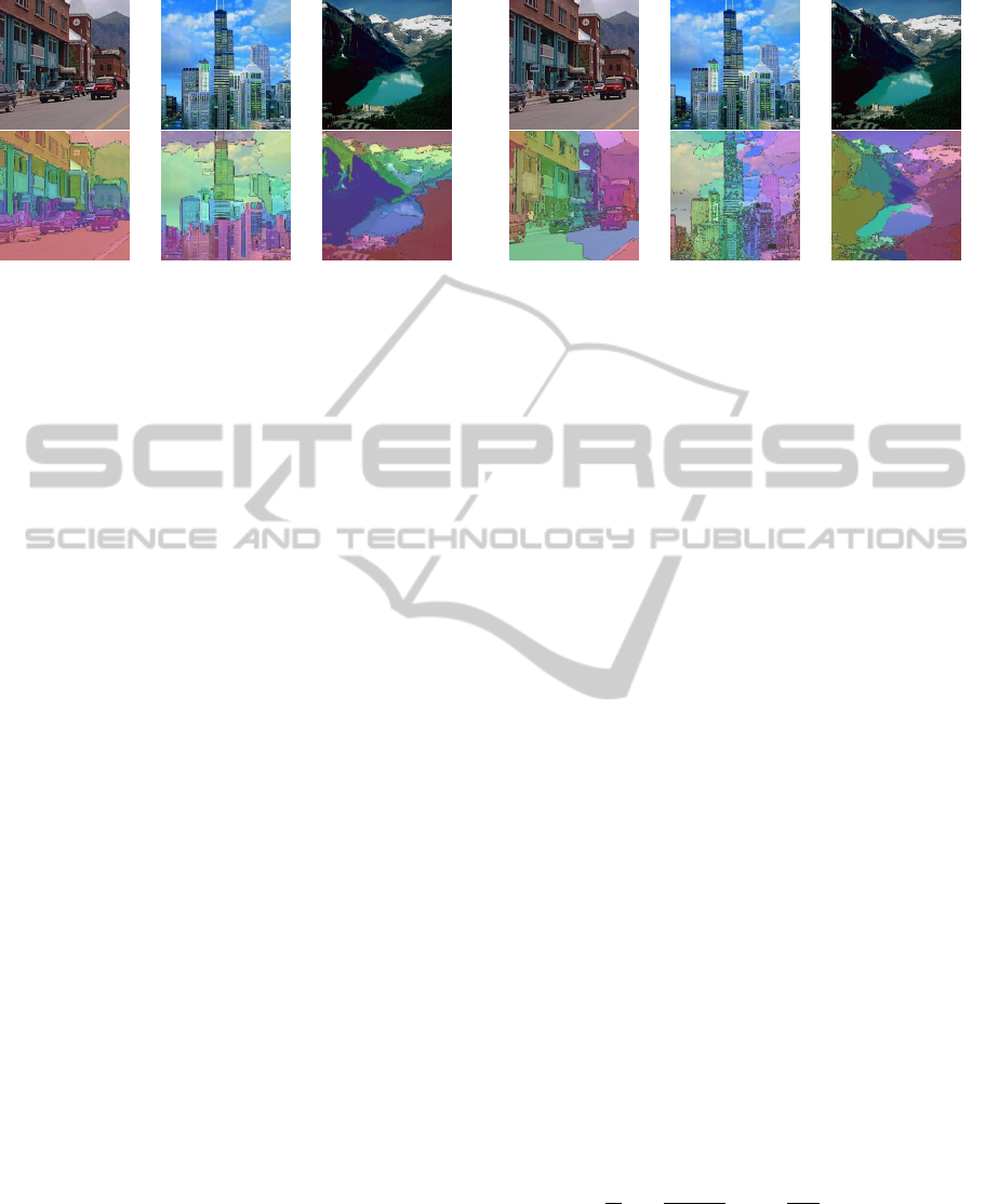
Figure 2: Visualization of the efficient graph-based image
segmentation on three images of the SIFT Flow database.
The parameters are set to ς = 0.8, w
g
= 200, t = 100.
graph G = (V,E) where the nodes v
i
∈ V represent
the pixels and neighboring pixels are connected by
edges (v
i
,v
j
) ∈ E. The edges connect the pixels in
a 4-connected neighborhood. In addition, a weight
ω(e) for an edge e ∈ E is calculated, which is defined
by the Euclidean distance between their color values.
A segment of an image can be described as a par-
tition Q ∈ V which forms a connected subgraph. The
approach is initialized by defining each pixel as its
own connected subgraph. Then similar subgraphs are
merged based on their internal differences and the dif-
ference to neighboring subgraphs. Typically, the im-
age is smoothed by Gaussian smoothing using a pa-
rameter ς beforehand.
As a segment should consist of pixels with similar
color values, the internal difference is defined as the
maximum edge weight of the minimum spanning tree
(MST, (Fredman and Willard, 1994)):
IntDi f (Q) = max
e∈MST (Q,E)
ω(e). (1)
Similarly the difference between two subgraphs can
be computed by
ExtDi f (Q
1
,Q
2
) = min
v
i
∈Q
1
,v
j
∈Q
2
,(v
i
,v
j
)∈E
ω(v
i
,v
j
), (2)
which represents the lowest weight of any edge be-
tween those two components. In case that two sub-
graphs do not share an edge, the weight is set to infin-
ity. In order to account for the size of different sub-
graphs, a normalization factor w
g
is introduced so that
the minimal internal difference of two subgraphs is
computed by
MIntDi f (Q
1
,Q
2
) = min(IntDi f (Q
1
) + τ(Q
1
),
IntDi f (Q
2
) + τ(Q
2
)) (3)
where τ(Q) = w
g
/|Q| with |Q| being the pixel count
of the subgraph. This implicitly models a desired size
for the segments that are created, since the internal
difference of two large subgraphs will be assigned a
Figure 3: Visualization of the Quick Shift on three images
of the SIFT Flow database. The parameters are set to σ =
10, τ = 30 and w
q
= 0.05.
high distance value. Two connected subgraphs are
merged if the external difference is smaller than the
minimal internal difference of those two subgraphs:
ExtDi f (Q
1
,Q
2
) ≤ MIntDi f (Q
1
,Q
2
).
Furthermore, in order to avoid the generation
of very small segments a parameter t is introduced
that defines a minimal component size. In a post-
processing step it enforces that components with less
than t pixels are joined with their nearest neighbor.
An illustration of superpixels created by the
graph-based segmentation algorithm is shown in
Fig. 2. You can see that this method tends to create
a quite cluttered over-segmentation with superpixels
of varying sizes and irregular shapes.
2.2 Quick Shift
The idea of Quick Shift (Vedaldi and Soatto, 2008)
originates from the Mean Shift algorithm and is based
on gradient descent. Mean Shift is initialized by es-
timating the modes of the data using a parzen den-
sity estimation. Then iteratively within each partition
the means are computed and the modes are shifted to-
ward the means (Comaniciu and Meer, 2002). Quick
Shift is a faster more efficient approach. Instead of
approximating the gradient, it estimates the mode by
connecting each point to the nearest neighbor.
Considering each pixel as a 5 dimensional fea-
ture consisting of its position and color value in the
L
∗
a
∗
b
∗
-color space. The parzen density estimate for
pixel i,
ρ(i) =
1
N
N
∑
j=1
1
(2πσ)
5
exp(−
1
2σ
2
d
q
(i, j)) , (4)
is computed. Then a tree is constructed by connecting
each pixel to its nearest neighbor with greater density.
The neighbors are considered within a spatial distance
depending on the Gaussian Kernel of standard devia-
VISAPP2015-InternationalConferenceonComputerVisionTheoryandApplications
520

tion σ. The tree is efficiently created by indexing:
ϕ
i
(1) = argmin
j:ρ( j)>ρ(i)
d
q
(i, j) (5)
The distances are computed by a weighted Euclidean
distance in the spatial and color domain
d
q
(i, j) = d
xy
(i, j) + w
q
· d
lab
(i, j) (6)
where w
q
is a weighting parameter. The smaller the
weight the more important is the spatial domain.
The algorithm would connect all pixels in one
large tree. Hence, a maximum distance τ is intro-
duced, splitting branches of the tree that have a higher
distance than τ. These splitted branches are then used
in order to create the superpixels.
An illustration of superpixels created by the Quick
Shift algorithm is shown in Fig. 3. Very similar to the
graph-based approach a set of superpixels of varying
sizes and shapes is created.
2.3 Simple Linear Iterative Clustering
The superpixel computation in the Simple Linear Iter-
ative Clustering (SLIC) method (Achanta et al., 2012)
is based on a grid-structured segmentation followed
by iterative clustering. It is initialized by placing a
set of centroids in the image based on a dense grid.
Hence, the first required parameter is the desired num-
ber of superpixels K. Ideally, the image should be di-
vidable in K equally sized grid cells. The centroid of
each grid cell is then moved toward the pixel with the
lowest local gradient in the local neighborhood, e.g.
3 × 3px, in order to be quite stable. Then, the assign-
ment of pixels toward a centroid is computed and the
centroids are updated. This process is repeated itera-
tively, similar to Lloyd’s algorithm.
The assignment of a pixel i to the centroids k is
computed based on minimizing the distance function
d
s
(i,k) = d
lab
(i,k) +
w
s
p
|I
I
I|/K
d
xy
(i,k) (7)
where |I
I
I| is number of pixels in the image I
I
I and d
xy
a
geometric term that represents the Euclidean distance
between the position of pixel i and centroid k. The
distance d
lab
is a color term that is defined by the Eu-
clidean distance between the color of the centroid k
and a given pixel i in the L
∗
a
∗
b
∗
-color space. Further-
more, w
s
is a weighting parameter. The higher the
weighting on the geometric term is the more square-
like the superpixels get. The update of the cluster cen-
ters is computed by the mean of the pixels assigned to
the respective cluster.
An illustration of superpixels created by SLIC is
shown in Fig. 4. You can see the influence of the
weighting parameter w
s
as well as the grid-based ini-
tialization influencing the over-segmentation to tend
toward a more uniform arrangement of superpixels.
Figure 4: Visualization of the SLIC algorithm on three im-
ages of the SIFT Flow database. The parameters are set to
K = 60 and w
s
= 1; w
s
= 10; w
s
= 50 (from left to right).
3 SUPERPIXELS FROM EDGE
AVOIDING WAVELETS
In this section a method for computing an over-
segmentation based on edge-avoiding wavelets (Fat-
tal, 2009) is proposed. A wavelet-transform can be
used to analyze frequencies of images in different
scales. A method which uses wavelets is the multi-
scale analysis.
A multi-scale analysis can be computed in order
to analyze an image by filtering high and low fre-
quencies while scaling the input signal, cf. (Gonzalez
and Woods, 2002). For a given input signal L
0
with
the highest resolution, the low-pass filtered and scaled
signal can be written as L
1
, where L
1
⊂ L
0
. The in-
put signal can be reconstructed, using the high-pass
filtered and scaled signal H
0
, which represents the
wavelet transformed signal, by L
0
= L
1
⊕ H
0
. With
the multi-scale analysis the signal is processed till
the highest possible scale r, with the lowest resolu-
tion, such that the input data can be reconstructed by
L
0
= L
r
⊕ H
r−1
⊕ H
r−2
... ⊕ H
0
.
An algorithmic approach to such a multi-scale
analysis is based on the so-called lifting scheme,
which is shortly described in section 3.1. The lifting
scheme applies a multi-scale analysis on a given one
dimensional signal without using an implicit wavelet
transform. An extension to two dimensional signals
such as images are red-black wavelets. This approach
is described in section 3.2.
While the lifting scheme and red-black wavelets
analyze the input data uniformly, the edge-avoiding
wavelets approach uses edge information in or-
der to compute image dependent wavelet functions.
The description of the computation of edge-avoiding
wavelets, using an image-dependent weight function,
can be found in section 3.3.
OntheInfluenceofSuperpixelMethodsforImageParsing
521

By exploiting the edge-avoiding properties of this
weight function at a given scale L
j
, inverse lifting can
be used for reconstructing the edge-avoiding scaling
functions in order to create an over-segmentation, as
described in section 3.4.
3.1 Lifting Scheme
The idea of the lifting scheme (Sweldens, 1998) can
be described in three steps: 1. The input signal is
split into two subsignals, initializing a scaling of the
signal. 2. In the prediction step the failure, resulting
from a simple splitting is predicted by adding infor-
mation from neighboring pixels from one subsignal to
another. 3. In the update step the scaled low-pass fil-
tered signal is created by adding information from the
predicted subsignal to the unprocessed (sub-)signal.
Splitting. The input signal, e. g., a discrete one di-
mensional time-depending signal L
j
, is split into its
odd and even coordinates, as is illustrated in Fig. 5.
The odd components are used for the extraction of the
low-pass filtered signal L
j+1
, whereas the even com-
ponents are mainly part of the high-pass filtered signal
H
j
. The corresponding indexing functions a and b are
defined by
a(i) = 2i − 1, b(i) = 2i, (8)
where i ∈ [1,...,N/2] and N being the index size of
the signal. Splitting a signal into parts as done so far
does apply a scaling but does neither apply a filter nor
does it take care about information loss. In order to
do so, two further steps, the prediction and the update
step, are employed.
Prediction. Using a prediction function R(i), the
high-pass filtered signal
H
j
(i) = L
j
(b(i)) + R(i) (9)
can be constructed, where
R(i) = −
1
2
(L
j
(a(i)) + L
j
(a(i + 1))) (10)
is using the neighboring data points in L
j
. With the
subtraction of the mean values the failure of the sim-
ple splitting step can be compensated and thus the de-
tails, i.e., the high-pass filtered signal can be calcu-
lated.
Update. Similarly to the prediction step, the update
step is used to eliminate a possible alias effect and
apply a low-pass filter by using the update function U
-1/2 -1/2 -1/2 -1/2
-1/2
-1/2
1/41/4
1/4 1/4
L
0
H
0
L
1
L
2
H
1
1/21/2 1/2 1/2
1/21/21/2
-1/4
-1/4
-1/4 -1/4
1/2
L
0
H
0
L
1
L
2
H
1
}
}
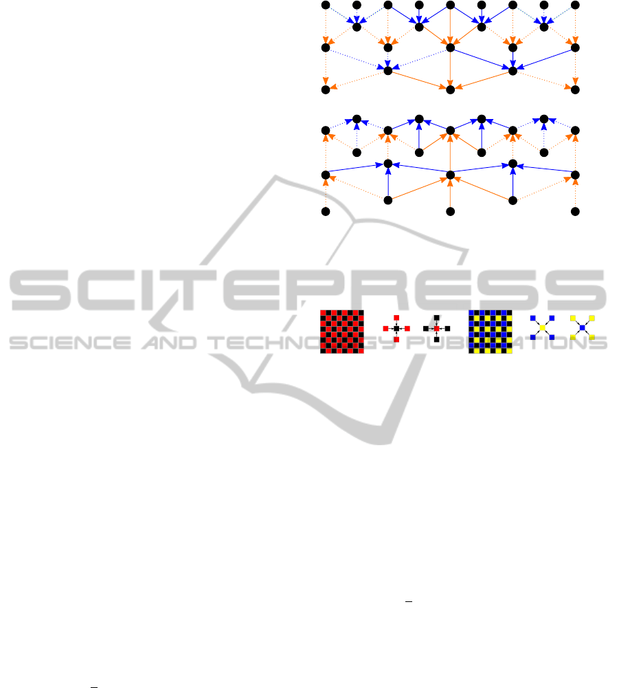
Figure 5: Overview of the lifting scheme: Top: Lifting is
applied on the signal L
0
, represented as black dots in the
top row. Blue arrows visualize the prediction step. Orange
arrows illustrate the update procedure. Bottom: Visualiza-
tion of the inverse lifting. Weights are negated.
Prediction I Update I
(a)
Prediction II Update II
(b)
Figure 6: Visualization of the red-black wavelet scheme: (a)
In the first iteration, pixels are split into red and black pix-
els. The prediction and update steps are processed using the
corresponding vertical and horizontal neighbor pixels. (b)
The second iteration splits the pixels into blue and yellow
pixels. Prediction and update steps are processed using the
corresponding diagonal neighbor pixels.
on the high-pass filtered signal. The low-pass filtered
signal results in
L
j+1
(i) = L
j
(a(i)) +U(i), (11)
where the update function is defined by
U(i) =
1
4
(H
j
(b(i − 1)) + H
j
(b(i))). (12)
One benefit of the lifting scheme is the possibility to
invert the scheme. As illustrated in Fig. 5, the inverse
lifting scheme can be easily achieved by traversing
the steps backwards while inverting the weights.
3.2 Red-black Wavelets
The lifting scheme can also be used on images. One
known method is called red-black wavelets, intro-
duced in (Uytterhoeven and Bultheel, 1997). The red-
black wavelets can be described as a two fold itera-
tion of the splitting, prediction and update steps. In
the first step, the image pixels are divided into even
and odd pixels, visualized as red and black pixels in
Fig. 6. For further simplicity a weight function ω
r
VISAPP2015-InternationalConferenceonComputerVisionTheoryandApplications
522

for neighboring pixels is introduced, which is used
for the prediction and update steps. Furthermore, let
I
I
I denote the given image and I
I
I
0
be the transformed
image, which in the beginning is equal to the input.
The first prediction step is applied on the black
pixels i, where the negative weighted mean of the red
pixels j in the neighborhood Γ
i
of pixel i is taken as
the prediction function
R(i) = −
∑
j∈Γ
i
ω
r
(I
I
I
0
(i),I
I
I
0
( j))I
I
I
0
( j)
∑
j∈Γ
i
ω
r
(I
I
I
0
(i),I
I
I
0
( j))
, (13)
with ω
r
being a weighting term. The new generated
black pixels are therefore calculated by
I
I
I
0
(i) = I
I
I
0
(i) + R(i). (14)
The following update step works similarly, but takes
the positive half of the weighted mean of the black
neighboring pixels as the update function
U(i) =
∑
j∈Γ
i
ω
r
(I
I
I(i), I
I
I( j))I
I
I
0
( j)
2
∑
j∈Γ
i
ω
r
(I
I
I(i), I
I
I( j))
, (15)
which results in
I
I
I
0
(i) = I
I
I
0
(i) +U(i). (16)
Note that the weight function ω
r
in the update step
depends on the original data. Although not impor-
tant here, it will be relevant for the edge-avoiding
wavelets.
In a second iteration, the image is split further into
blue and yellow pixels, as illustrated in Fig. 6. The
prediction step is applied on the yellow pixels with
blue pixels as neighbors, while afterwards the blue
pixels are updated with the yellow neighboring pix-
els. The resulting image can be interpreted as follows:
Blue pixels represent the low-pass filtered, scaled im-
age. Yellow pixels are storing the diagonal detail in-
formation, whereas the black pixels represent the hor-
izontal and vertical details.
3.3 Edge-avoiding Wavelets
Red-black wavelets, also known as the second genera-
tion wavelets are using homogeneous weights to filter
the data. Another approach is used in (Fattal, 2009).
The edge-avoiding wavelet technique uses weights,
depending on the difference in the intensity of pixel
neighbors. The calculation of the differences in this
case is a retrieval of edge information. This procedure
makes the analysis dynamic, depending on the given
image data. The weight function ω
r
for neighboring
pixel values m and n is defined by the equation
ω
r
(m,n) = (|m − n|
α
+ ε)
−1
, (17)
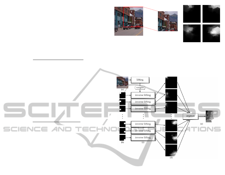
(a) (b)
Figure 7: Given an image (a) the edge-avoiding wavelets (b)
are limited by borders inside the image. The shown weight
matrices (b) represent four inverse lifted scaling functions
at the image section, illustrated in (a).
Figure 8: Segmentation, using edge-avoiding wavelets: (a)
The input image is being processed with the lifting scheme.
(b) For a chosen scale, images of the corresponding reso-
lution are created, where only one pixel per image is set to
one. (c) An inverse lifting with the previously calculated
weights, applied to the created images, creates the weight
matrices (d) with the resolutions of the input image. (e) An
argmax function calculates the superpixels, visualized by
different grey values.
where α is a weighting parameter. Further process-
ing steps follow the red-black wavelet algorithm, as
described above. As Fig. 7 visualizes, edges are
avoided, using the edge information for weighting the
prediction and update steps in the red-black wavelets.
Hence, it is important that the update always depends
on the edges from the original data.
3.4 Superpixel Computation
The idea behind calculating superpixels from edge-
avoiding wavelets is based on the scalability and the
edge restriction of these wavelets. Superpixels should
cover areas which are limited by edges, this can be a
change in color, which is why edge-avoiding wavelets
are a good option to compute regions. The construc-
tion of the superpixels, illustrated in Fig. 8, can be de-
OntheInfluenceofSuperpixelMethodsforImageParsing
523

scribed in three processing steps lifting, inverse
lifting and merging:
First, the lifting step is analyzing the given image
with the edge-avoiding wavelets as described in sec-
tion 3.3. All weights, calculated for each scale and
prediction or update steps are stored. Second, one
scale l and the corresponding resolution of the low-
pass filtered signal L
l
are chosen to define the amount
of superpixels to calculate, corresponding to the num-
ber of blue pixels (see Fig. 6). Third, for each super-
pixel s
i
, an image L
0
l
with the resolution of L
l
of the
chosen scale l is constructed, where one pixel is set
to one, while the rest is set to zero. This represents a
grid-like initialization of the superpixel computation
so that the number of superpixels K is defined by the
number of pixels in L
l
. These initial images L
0
l
are
now handled as low-pass filtered images at the given
scale, replacing the detail coefficients. Given these
images the inverse lifting scheme is applied for all of
them by using the stored weights, but not the detail
coefficients, to construct a weight matrix W
W
W
j
for each
image with the resolution of the original image. The
weighting clouds grow, starting at the initial point of
the selected scale. Being in the range [0,1], high val-
ues indicate a region, while the edges are indicated by
an abrupt change of intensity.
In the final merging step we use the weight ma-
trices to calculate superpixels. This is done by an
argmax operation over all weight matrices W
W
W
j
, where
the argument is defined by the index j. The values of
the constructed superpixel indexing matrix Y
Y
Y can be
described as
Y
Y
Y (i) = argmax
j
(W
W
W
j
(i)), (18)
for all points i of the image I
I
I. Each value represents a
superpixel classification. As the argmax function can
cause parts of the superpixels to be unconnected to
the main region, a further post-processing step is used
to relabel these unconnected regions by joining them
with the largest adjacent superpixel.
A visualization of the segmentation through edge-
avoiding wavelets without relabeling unconnected su-
perpixels is shown in Fig. 9 for 2 × 2, 4 × 4 and
8 × 8 superpixels, where the last one already yields
a superpixel-like over-segmentation. As can be seen,
the superpixels are placed grid-structured, while the
region’s shape is defined by edges in the image.
4 EVALUATION
The different superpixel methods were evaluated on
two large datasets. First, the SIFT Flow database
Figure 9: Visualization of the segmentation based on edge-
avoiding wavelets (with partially unconnected regions of
one superpixel) on three images of the SIFT Flow database.
The parameters are set to α = 1 and K = 4, 8 and 64 respec-
tively (from left to right).
(Liu et al., 2011) and second the Barcelona database
(Tighe and Lazebnik, 2010) are evaluated. The
SIFT Flow database contains 2688 images of natu-
ral scenes and 200 of those are defined as the test-
set. The dataset contains 33 different categories. The
Barcelona database contains 14871 images of which
279 are used for the testset. While the whole set con-
tains of a wide range of scenes, the testset is created
from scenes located in Barcelona giving the dataset its
name. The dataset contains 170 different categories.
4.1 Evaluation Setup
The evaluation builds on the Superparsing setup from
(Tighe and Lazebnik, 2010; Tighe and Lazebnik,
2013b). Here, in all experiments the retrieval set
consists of the 200 Nearest Neighbors using different
global feature representations. The labels for the su-
perpixels are computed based on the 80 most similar
superpixels using Z local feature types. A descrip-
tion and evaluation of the different features represen-
tations is given in (Tighe and Lazebnik, 2013b). The
probabilities for the superpixel s
i
to belong to class c
is then computed by
γ(s
i
,c) =
∏
m
P( f
z
i
|c)
P( f
z
i
|c)
(19)
assuming that the features f
z
i
are independent. Here,
for each feature type the probability for a given class
is computed by
P( f
z
i
|c)
P( f
z
i
|c)
=
(κ(c,N
m
i
)+ε)/κ(c,D)
(κ(c,N
m
i
)+ε)/κ(c,D)
=
κ(c,N
z
i
)+ε
κ(c,N
z
i
)+ε
×
κ(c,D)
κ(c,D)
(20)
where c denotes the class label and c is the set of
classes excluding c. N
z
i
denotes the set of superpix-
els that were retrieved from the most similar images
VISAPP2015-InternationalConferenceonComputerVisionTheoryandApplications
524

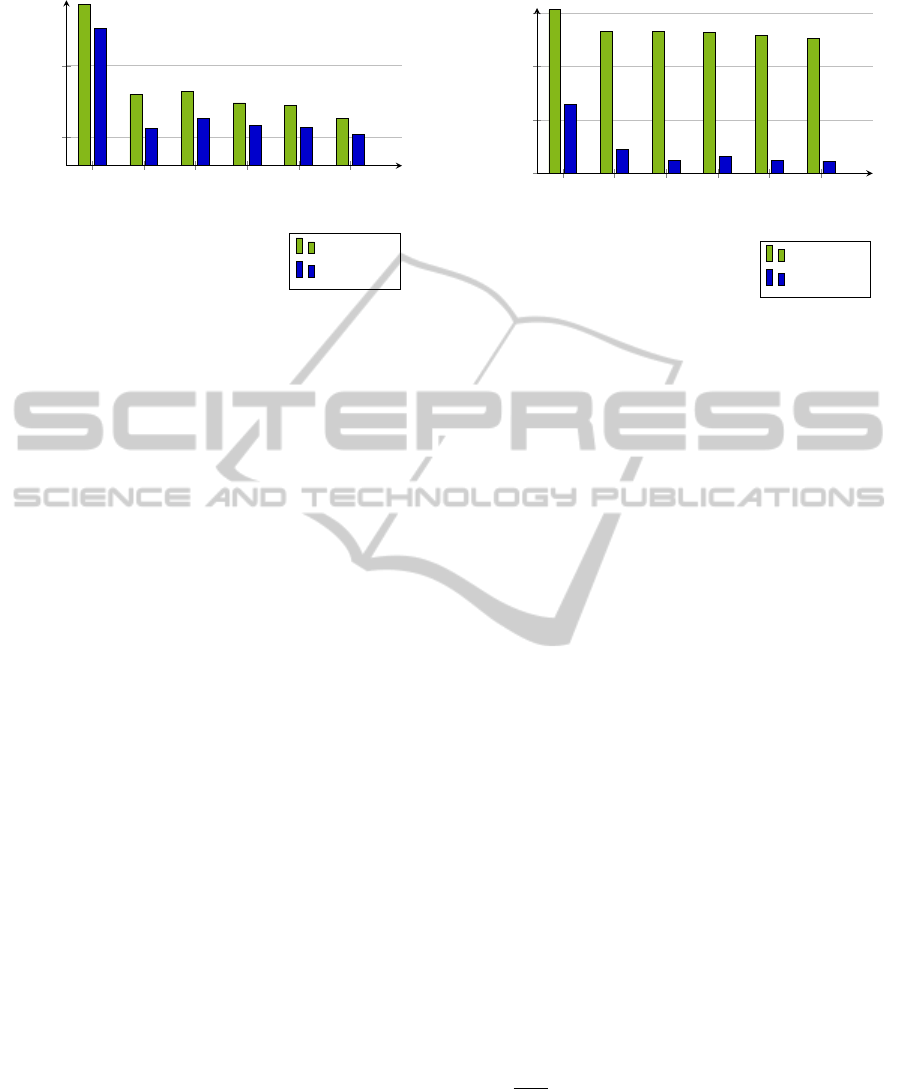
Ground Truth
Graph-based
SLIC
Quick Shift
EAW
Grid
85
90
accuracy [%]
Pixelwise
Classwise
Figure 10: Evaluation of different superpixel methods for
the geometric labels (vertical, horizontal, sky) of the SIFT
Flow database. For comparison a ground truth segmentation
that corresponds to the semantic classes of the dataset as
well as a simple grid are shown. The results are shown for
a pixelwise and a classwise evaluation.
for query superpixel s
i
in feature representation k. D
denotes all superpixels of the training set. So that
κ(c,S) is the count of all superpixels with label c in
the respective set. The constant ε is added for smooth-
ing in order to avoid zero probabilites. The labels for
the training set are obtained by labeling the superpixel
with the label most frequently occuring in the ground
truth. If less than 50% of a superpixel have one la-
bel so that no clear majority is observed in the anno-
tations this superpixel is discarded from the training
and, therefore, from the retrieval sets.
As the focus of the evaluation is on the influence
of the superpixel algorithms, no additional extensions
of the algorithms, such as the inference between ge-
ometric and semantic labels, the contextual inference
between neighboring regions or the object detectors,
are considered.
The Superparsing method was evaluated in com-
bination with the three superpixel methods discussed
in section 2 and the proposed method described in
section 3. The efficient graph-based segmentation,
described in section 2.1, has also been applied in
the original publication. For further evaluation the
ground truth annotations are used in order to obtain
a semantically correct labeling. These labels should
indicate an upper bound for the recognition rate. Ad-
ditionally, a grid is evaluated as the simplest possible
solution for an image segmentation. It also poses the
most efficient way as it is very easy to compute.
The parameters of the superpixel methods were
evaluated on the SIFT Flow dataset and the best con-
figuration has then also been applied to the Barcelona
dataset. The pixel- and classwise recognition rates
have been evaluated. Note that large uniform re-
gions strongly influence the pixelwise recognition
Ground Truth
Graph-based
SLIC
Quick Shift
EAW
Grid
20
40
60
80
accuracy [%]
Pixelwise
Classwise
Figure 11: Evaluation of different superpixel methods for
the semantic labels of the SIFT Flow database. For com-
parison a ground truth segmentation that corresponds to the
semantic classes of the dataset as well as a simple grid are
shown. The results are shown for a pixelwise and a class-
wise evaluation.
rates while small objects and under-represented cat-
egories strongly influence the classwise recognition
rates.
4.2 SIFT Flow Dataset
For all methods an extensive evaluation has been per-
formed, deciding on the best parameters. The setups
with the best pixelwise classification rates have been
chosen for further comparison. Note that the opti-
mization will result in comparably good results for
most methods, while a non-optimal choice of param-
eters will cause the recognition rates to deteriorate.
For the size of the grid an optimal size has been
found using 11× 11 tiles. The finer the grid is the bet-
ter the classwise accuracy becomes, but the per pixel
rate is deteriorating at scales finer than 11 × 11.
For the graph-based segmentation the image is
smoothed by ς = 0.8, the weighting parameter for
merging components is set to w
g
= 200 and the mini-
mum segment size to t = 100, as in (Tighe and Lazeb-
nik, 2013b). The minimum segment size t discards
smaller superpixels, yielding around 64 superpixels.
For SLIC the desired number of superpixels is set
to K ≈ 50, for a grid-like initialization this equals
K = 7 × 7 and a weight of w
s
= 1, which puts a higher
weight to the pixel distance than to the color distance
(w
s
/
p
1/K ≈ 7). However, the value range of the
color distance in L*a*b* space can be much higher
than the pixel distances, so that it does not cause the
superpixels to be completely square-like.
The Quick Shift parameterization uses a Gaussian
window with standard deviation σ = 10 and a maxi-
mum pixel distance τ = 30. The weight w
q
is set in
OntheInfluenceofSuperpixelMethodsforImageParsing
525

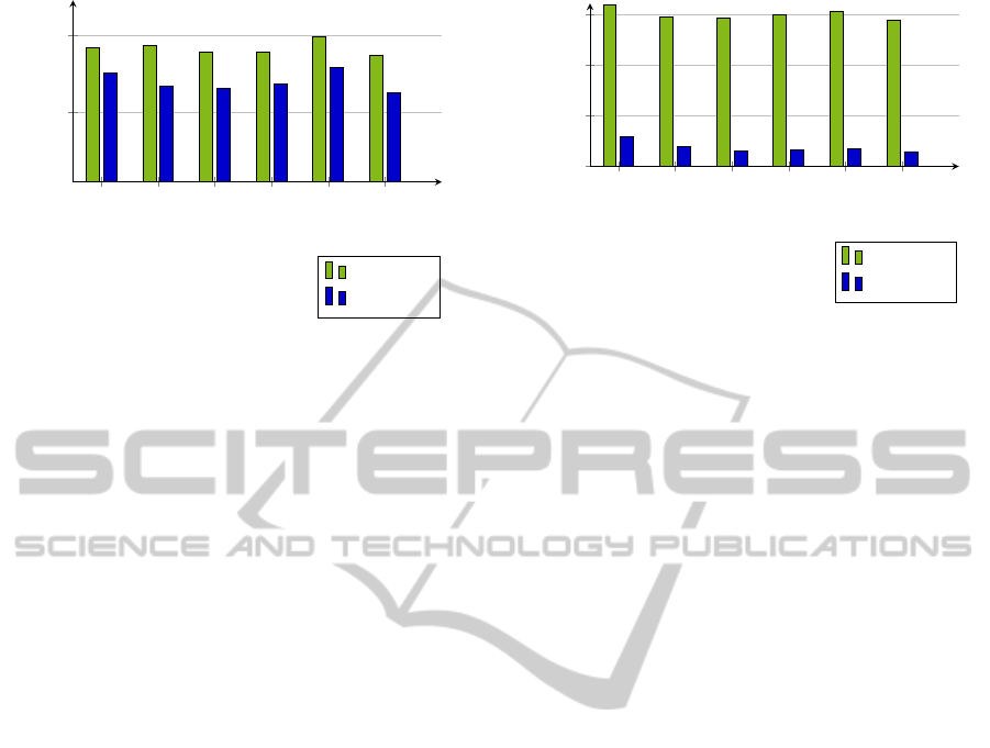
Ground Truth
Graph-based
SLIC
Quick Shift
EAW
Grid
80
90
accuracy [%]
Pixelwise
Classwise
Figure 12: Evaluation of different superpixel methods
for the geometric labels (vertical, horizontal, sky) of the
Barcelona database. The results are shown for a pixelwise
and a classwise evaluation.
favor of the spatial domain with w
q
= 0.05, similarly
to the SLIC weight.
For the edge-avoiding wavelet based approach
(EAW) K = 256 so that 16×16 pixel images are used
for initializing the inverse lifting for a 256 × 256px
image as given in the SIFT Flow database. For im-
ages of different sizes and aspect ratios the number of
superpixels will change respectively. The weighting
for the red-black wavelets is set to α = 1.
Considering these parameters, it is interesting that
depending on the typical shapes that are produced by
the different superpixel methods, an optimal number
of superpixels is varying between 49 and 256.
The final performance of these methods is shown
in Fig. 10 for the three geometric classes and in
Fig. 11 for the 33 semantic classes. Here, it can
be seen that the graph-based image segmentation is
a good choice for the classwise accuracy of the se-
mantic classes. However, in all other measures it is
outperformed by SLIC.
This can be explained by the fact that the graph-
based image segmentation is more cluttered than, for
example, the results of SLIC or the edge-avoiding
wavelet based approach, which are initialized by a
grid-like structure. It is more likely for the graph-
based segmentation to cover small objects, larger ar-
eas will not be captured that well and noise will be
introduced. Therefore, the proposed edge-avoiding
wavelet approach performs comparably well on the
geometric labels where the labeled areas are typically
larger due to the smaller number of classes.
The comparison to the ground truth segments
shows that a semantically correct segmentation im-
proves the results of all measures. This indicates
that better segmentation algorithms would improve
Ground Truth
Graph-based
SLIC
Quick Shift
EAW
Grid
0
20
40
60
accuracy [%]
Pixelwise
Classwise
Figure 13: Evaluation of different superpixel methods for
the semantic labels of the Barcelona database. The results
are shown for a pixelwise and a classwise evaluation.
the recognition rates of image parsing. Especially the
classwise recognition rates could benefit a lot.
The grid performs notably well, considering that
no effort went into the segmentation stage. The recog-
nition rates on the semantic labels is not far below
the results of the best segmentation method. Namely,
2.6% for the pixelwise recognition rate and 4.5% for
the classwise recognition.
4.3 Barcelona Dataset
For the Barcelona database the same parameters that
have been optimized on the SIFT Flow database have
been used. This dataset is more challenging, as there
are more semantic classes and cluttered scenes from
the streets of Barcelona.
The results for the geometric and semantic labels
are shown in Fig. 12 and Fig. 13 respectively. Again
the graph-based segmentation performs good on the
classwise measure for the semantic classes, although
the difference is quite small. However, SLIC and es-
pecially the edge-avoiding wavelet based segmenta-
tion performs well on all other measures. The scenes
are cluttered, but also contain several man made struc-
tures that can be covered quite well by the edge-
avoiding properties of this approach. On the semantic
classes a recognition rate of 61.2% is achieved. With
a pixelwise recognition rate of 89.9% on geometric
labels even the ground truth segments that show only
88.4% are outperformed. Henceforth, proofing the
necessity of an over-segmentation, but also showing
the advantage of less noisy segments compared to the
graph-based segmentation. With respect to the pos-
sible extensions, a high recognition rate of geomet-
ric classes would also be beneficial for improving the
results by inference between semantic and geometric
classes as described in (Tighe and Lazebnik, 2013b).
VISAPP2015-InternationalConferenceonComputerVisionTheoryandApplications
526

Considering the effort that is nowadays used in
order to improve the recognition rates on these dif-
ficult image parsing tasks, it shows how important
the choice of the segmentation algorithm is. There
is not necessarily an optimal choice for all tasks, but
depending on the focus of the application it could be
shown that superior results to the de-facto standard
can be achieved.
5 CONCLUSION
In this paper an evaluation of different superpixel
methods in an image parsing framework has been
shown and an over-segmentation approach that is
based on edge-avoiding wavelets has been proposed.
The evaluation has been performed on two large im-
age parsing datasets, the SIFT Flow and the Barcelona
database. It showed the advantages and disadvantages
of different superpixel approaches.
The choice of the superpixel method and their
properties are quite important for the performance of
the image parsing. Instead of relying on one method,
different methods should be chosen with respect to the
task that has to be optimized. Smaller more noisy seg-
ments typically perform better for capturing a large
set of different classes that do not cover large areas of
the image. Here, especially the graph-based segmen-
tation showed good results for the classwise evalua-
tion. For an overall correct annotation on pixel-level
or a smaller set of classes that cover larger areas of
the image the superpixel methods that create more
stable and slightly more uniform regions perform bet-
ter. Here, especially SLIC and the proposed edge-
avoiding wavelet based approach show good results
as their initialization is related to a grid-like structure.
The proposed edge-avoiding wavelet method
showed very promising results on the geometric la-
bels where only a few sets of classes are consid-
ered as well as on the pixelwise semantic labeling.
This demonstrates that the stable regions as well
as the edge-avoiding properties yield a useful over-
segmentation of natural scenes. Due to the nature of
the lifting scheme, the method could also be extended
to a multi-scale approach.
REFERENCES
Achanta, R., Shaji, A., Smith, K., Lucchi, A., Fua, P., and
S
¨
usstrunk, S. (2012). SLIC superpixels compared to
state-of-the-art superpixel methods. IEEE Transac-
tions on Pattern Analysis and Machine Intelligence,
34(11):2274–282.
Badino, H., Franke, U., and Pfeiffer, D. (2009). The
stixel world-a compact medium level representation
of the 3d-world. In Pattern Recognition, pages 51–
60. Springer.
Comaniciu, D. and Meer, P. (2002). Mean shift: A robust
approach toward feature space analysis. IEEE Trans-
actions on Pattern Analysis and Machine Intelligence,
24(5):603–619.
Farabet, C., Couprie, C., Najman, L., and LeCun, Y.
(2013). Learning hierarchical features for scene la-
beling. IEEE Transactions on Pattern Analysis and
Machine Intelligence, 35(8):1915–1929.
Fattal, R. (2009). Edge-avoiding wavelets and their ap-
plications. ACM Transactions on Graphics (TOG),
28(3):22.
Felzenszwalb, P. F. and Huttenlocher, D. P. (2004). Effi-
cient graph-based image segmentation. International
Journal of Computer Vision, 59(2):167–181.
Fredman, M. L. and Willard, D. E. (1994). Trans-
dichotomous algorithms for minimum spanning trees
and shortest paths. Journal of Computer and System
Sciences, 48(3):533–551.
Gonzalez, R. C. and Woods, R. E. (2002). Digital image
processing. Prentice Hall.
Liu, C., Yuen, J., and Torralba, A. (2011). Nonparamet-
ric scene parsing via label transfer. IEEE Transac-
tions on Pattern Analysis and Machine Intelligence,
33(12):2368–2382.
Neubert, P. and Protzel, P. (2012). Superpixel benchmark
and comparison. In Proc. Forum Bildverarbeitung.
Sweldens, W. (1998). The lifting scheme: A construction of
second generation wavelets. SIAM Journal on Mathe-
matical Analysis, 29(2):511–546.
Tighe, J. and Lazebnik, S. (2010). Superparsing: Scal-
able nonparametric image parsing with superpixels.
In Proc. European Conference on Computer Vision
(ECCV), pages 352–365. Springer.
Tighe, J. and Lazebnik, S. (2013a). Finding things: Im-
age parsing with regions and per-exemplar detectors.
In Proc. IEEE Conf. on Computer Vision and Pattern
Recognition (CVPR), pages 3001–3008. IEEE.
Tighe, J. and Lazebnik, S. (2013b). Superparsing.
International Journal of Computer Vision (IJCV),
101(2):329–349.
Uytterhoeven, G. and Bultheel, A. (1997). The red-black
wavelet transform. TW Reports.
Vedaldi, A. and Soatto, S. (2008). Quick shift and ker-
nel methods for mode seeking. In Computer Vision–
ECCV 2008, pages 705–718. Springer.
OntheInfluenceofSuperpixelMethodsforImageParsing
527