
A New Approach for the Detection of Emergent Behaviors and
Implied Scenarios in Distributed Software Systems
Extracting Communications from Scenarios
Fatemeh Hendijani Fard
and Behrouz H. Far
Department of Electrical and Computer Engineering, University of Calgary, Calgary, Canada
1 RESEARCH PROBLEM
An approach to specify the requirements and design
of a Distributed Software System (DSS), which is
mostly used in recent years, is describing scenarios
with visual artefacts, such as, UML Sequence
Diagrams and ITU-T (ITU-T UNION, 2004)
Message Sequence Charts (MSC) and High level
Message Sequence Charts (hMSC) (Krüger, 2000).
Scenarios describe system’s behavior and define the
components and their interactions. Each scenario
determines a partial behavior of the system. Hence,
the restricted view of the components in each
scenario and distributed functionality and/or control
in DSS, may result in inconsistency in the system
behavior.
One problem that arise in scenario based
Distributed Software Systems is emergent behaviors
or implied scenarios that occur because of restricted
view of one or more components. Emergent
behaviors are known as unexpected behaviors that
components show in their execution time (Uchitel,
2003; Bhateja et al., 2007). However, this behavior
was not defined in their designs. This unexpected
behavior may imply a new scenario to the system,
and can result in considerable cost and damage (Alur
et al., 2005). Therefore, emergent behaviors should
be detected in the early phases of software
development to prevent damage or cost after
deployment. The detected emergent behaviors can
be either accepted or denied by the stakeholders.
However, they should be detected and discussed, to
be added as new designs, or to be specified as
negative scenarios that should be avoided (Uchitel et
al., 2002).
In our research, we try to devise an automatic
methodology to detect the emergent behaviors
(implied scenarios) from the designs of the system.
We also mean to help the designers for the exact
point of the problem in the system and the possible
solutions to remove the detected emergent
behaviors.
2 OUTLINE OF OBJECTIVES
Many approaches in the literature are defined, for
the detection of emergent behaviors in early phases,
to save cost of fixing them after deployment. Some
of the approaches use formal methods and Finite
State Machine methodologies to construct the
behavior modeling of the components and verify
them against some properties.
Some of the issues with many methodologies
under this category are performance, their cost, the
amount of time for defining the constraints and
rules, besides expertise and knowledge required for
the applications and language notations or
techniques (Holzmann and Smith, 2002; Iglesias,
2009; Uchitel, 2009; Briand, 2010). Furthermore, in
the requirement model checking of scenarios, these
approaches cannot identify the exact location of the
scenario specification causing errors (Song et al.,
2011).
Some of the problems we have found during our
study are:
P1: The process of constructing behavioral models
is complex and hardly scalable. Therefore, it needs
special algorithms and tools to model components’
behavior besides the emergent behavior detection.
The process of behavioral modeling is time
consuming and complex (Mousavi, 2009).
P2: The existing methods using behavior modeling
are message dependent. This requires a great time
and effort to verify the specifications if system
requirements change, e.g. adding a new component
or modifying interactions between the existing
components. In this case, the whole process should
be done from the scratch. Besides, the message
dependency in this level requires domain expertise
to annotate the model or specify proper
specifications (Chaki et al., 2005)
P3: While system requirements especially in
scenario based systems show the interaction of all
types of components of the system, they can’t show
15
Hendijani Fard F. and H. Far B..
A New Approach for the Detection of Emergent Behaviors and Implied Scenarios in Distributed Software Systems - Extracting Communications from
Scenarios.
Copyright
c
2015 SCITEPRESS (Science and Technology Publications, Lda.)

this interaction among all instances for each type.
Therefore, emergent behavior can still exist between
some components of the same type (e.g. all sellers in
an online auction system are of the Seller type); but
existing research cannot handle this.
P4: Differentiating between send and receive
messages is not considered in many researches
(Song et al., 2011), or needs identifying specific
definitions to recognize between send and receive
messages between the components. While in real
world, send messages are not received at the
moment they are sent. This makes a flaw between
detecting emergent behaviors in requirement phase
and what really happens in system execution.
Specifically, we have the following research
objectives in our research:
O1: Classifying emergent behavior types in DSS.
O2: Devising a message content independent
technique for detection of a subset of classified
emergent behaviors of G1 in DSS addressing the P1-
P4 problems.
O3: Implementing a tool that can find emergent
behaviors in DSS and providing solution to the
research questions.
3 STATE OF THE ART
There is a lot of research that transform the MSCs or
SDs to various versions of state machines for the
detection of implied scenarios. Some research
present theorems on the complexity and decidability
of implied scenario detection in different
specifications, and in various communication
channels and styles (Alur et al., 2005; Bhateja et al.,
2007). Some other, provide tools to detect and
animate the labelled transition systems for implied
scenarios (Letier et al., 2005). (Chakraborty, et al.,
2010) mentions that some of these works are not
amendable or do not show correctness. A common
issue that exists in some methodologies is requiring
human input. For example in (Mousavi, 2009) the
domain expert should fill out some tables to define
the semantic causalities among various messages.
We try to solve this issue by using message labels
instead of message contents, and not using semantic
causality. Based on our knowledge, the only
different method is generating and comparing two
graphs for specification and implementation, which
shows the points that an implied scenario can occur,
without specifying clues for the designers (Song et
al., 2011).
4 METHODOLOGY
In our approach, the components’ communications
are modeled into interaction matrices, which is
inspired by social network analysis (SNA)
(Aggarwal, 2011), in which, the communications
among individuals are modeled and mined. In SNA,
the identities of the communicating individuals are
important (may be confidential and hidden in some
cases). Likewise, in our model, we try to keep the
processes’ labels (identities) in the interactions,
rather than just keeping the processes’ states. A
direct advantage of this modeling is saving all the
information about the communication of
components. This information, which is preserved
throughout the extracted vectors, is used as a clue
for the designer to examine the consequences of a
design decision and fix the detected emergent
behaviors. Another advantage of this modeling is
detecting warning points in processes’ interactions,
in terms of, giving the information about the sender
or receiver of a message, or hiding this type of
information. The warning points can help the
designers figure out the possible problems that are
effects of a design decision, and provide clues to the
designers on how to fix various issues.
This modeling is one step toward the
implementation of design decisions that guides the
designers to include necessary information in the
system designs. The other benefit of our modeling is
visualization of components’ interactions and their
state diagrams – by preserving information about
their interactions – that provides visual support for
the designers. The warning points and possible
problems can be illustrated in various diagrams,
which supply the information about the exact state,
MSC, and cause of the emergent behavior in the
system.
To overcome the problems mentioned in
previous sections, we have two main techniques in
our proposed methodology. First, we approach the
problem by identifying the components that will not
show an implied scenario. These components can be
omitted from further component level analyses. This
will help scalability of the component level implied
scenario detection (i.e. analyzing the behavior of
each component, without considering the other
components' behaviors in the system) (Fard and Far,
2013). Second, we have classified the implied
scenarios in various types. Until now, six main
categories are specified, based on the literature, and
our studies. To the best of our knowledge, this
classification is a contribution of our work. The
classification of common types of emergent
ICAART2015-DoctoralConsortium
16

behaviors can lead to better study the detection,
reasons behind each problem, and developing
solutions for each type of emergent behavior. The
six types that we have classified are:
TYPE TP1: Process p may have an implied
scenario when it has some shared states in two or
more MSCs and it sends one or more messages to
different processes in these MSCs. The send action
of process p can be in or after its shared states.
TYPE TP2: This type is similar to TP1. In this type,
the send actions of process p are a response to its
previous interactions with various processes, where
these interactions are exactly before or in shared
states of process p. This type is important in cases
that security or privacy issues should be
implemented. The interaction details of process p
may be shown in the designs, but should be hidden
in the implementations. Therefore, the design and
implementation are not equal. This difference, can
lead to an implied scenario.
TYPE TP3: Consider that process p is sending
messages in MSC M1 and process q is sending
messages in MSC M2. The combination of
projections of these MSCs is a new scenario M3 that
is implied to the system. In M3, which is not in the
designs, both processes p and q are sending
messages.
TYPE TP4: This class of implied scenario
originates from the asynchronous concatenation of
MSCs; a case that the processes perform their tasks
independently. In other words, a process may
proceed to the next MSC, while other processes are
still involved in the previous MSCs. Therefore, there
is no guarantee that all events in MSC M2 are
performed after all events in MSC M1, where M2 is
designed to execute after M1 in hMSC. We have
specified various subcategories of this type of
implied scenario and the situations that may result in
having TP4.
TYPE TP5: A sub category of TP4 is known as
non-local or branching choice. In this case, different
processes can follow different choices according to
the hMSC. However, the result is that some
processes follow a branch and the rest follow
another MSC. Consequently, the result is not in
accordance with any of the branching choices in the
hMSC. We have devised this type as a separate class
of implied scenarios because of the importance of
investigating the interactions of processes in
branching choices. We have found that, not all of the
processes can follow various branches in a
branching choice in hMSC. The processes that may
behave differently are the ones that start an
interaction in those MSCs and do not depend on
receiving some messages from other processes to
continue their actions. We call these active
processes.
TYPE TP6: The local visual order of process p is
not always preserved in the execution time.
Therefore, a change in the order of events on a
process life line can lead to TP6. A subcategory of
this type is known as race conditions. In race
conditions, two or more processes compete in
reaching a resource (sending a message to one
process in our case).
For each type, we specify the situations that can lead
to an implied scenario. Based on the required
information for the occurrence of each type,
different vectors are defined and extracted from the
models for the detection algorithms.
5 EXPECTED OUTCOME
The classification of common types of emergent
behaviors is based on the reasons and various
conditions that can lead to each case. Therefore, the
classification will help devising the detection
algorithms, specifically to each category, which can
also lead to suggest solutions on how to omit the
problem or change the designs to fix the detected
emergent behavior or implied scenario.
In this section, we focus on one of the emergent
behavior types (TP4) that can occur because of
asynchronous concatenation of MSCs. The
asynchronous concatenation of MSCs is interpreted
as concatenation of processes’ actions
independently. In other words, in an hMSC, one
process can proceed to the next MSC, while another
process is still involved in the previous MSC. The
asynchronous concatenation of MSCs can cause two
main problems that should be detected, in order to
prevent emergent behaviors. These two problems,
which we refer to as issues I1 and I2, are
investigated here. In general, for this type, the high
level structure
of each process is identified. This
structure is compared with the structure of hMSC.
The
of each active process, should have the same
loops, initial and final MSCs as the hMSC. If the
initial MSC of
for an active process is not the
same as initial MSC of hMSC, there is a chance to
emerge an implied scenario. The reason is that, the
active process can start to perform its actions
without depending on the other processes. Thus, this
process may start its tasks in its own initial MSC,
while the other processes are not performing the
ANewApproachfortheDetectionofEmergentBehaviorsandImpliedScenariosinDistributedSoftwareSystems-
ExtractingCommunicationsfromScenarios
17

same MSC, resulting in a new scenario that is not in
the hMSC of the system.
5.1 Definitions
The basic definitions required for our modeling are
described in this section.
5.1.1 Message Sequence Charts (MSC)
Let
,,,…
be the finite set of processes
(components, agents) of the system, which are
interacting with each other. We define ∑
as the set
of communications that process takes part in.
∑
!
,?
|
, ∈ , ∈
where is the finite set of messages on the system.
The !
defines that process sends message
to process , and ?
defines that process
receives message from process . We define
∑∪
∈
∑
.
Each MSC shows a visual form of processes
and their interacting messages over the finite set
of messages . An MSC is a structure
,,,,, where:
,
,… is a finite set of and
events, where
,
,… is the set of
events and
,
,… is the set of
events.
is a finite set of processes.
is a finite set of messages.
: → ∑ is a mapping function of events to
messages and processes. For ∈, ∈∑ and
∈:
|
∈∑
,
The set of events on process ∈ is:
|
∃ ∈ , ∈ ,
!
∈,
?
And
∪
∈
is the set of total orders on and .
: → maps the send events to receive events. For
,′ ∈ and , ∈ , we define:
≡∃ ∈
!
′
?
The
relation explains that the message
sent by at event is received by at event ′.
Each MSC has a visual structure showing the set
of processes interacting to each other via sending
or receiving messages. The process ∈ in an
MSC is shown by a vertical line representing the life
line of the process. The interacting messages are
shown with arrows (edges ) from one process to
another process. The events
on process have a
local visual order represented by
, which is the
total order of events on as displayed in the MSC.
The visual order of an MSC contains the
local orders of all processes and the set of all edges
on that MSC:
∪
∈
∪
5.1.2 High Level MSC
High level MSC (hMSC) is a structure
,,,,,∁,
,
, where is the set of
processes, is the set of messages, represents
the set of MSCs, represents the vertices, ⊆
is the set of edges, and ∁ is a mapping
function ∁: → . The
⊆ and
⊆ are the
initial and final vertices of .
For each process ∈ in , we define a
structure
,
,
,
,∁
,
,
,
where
⊆ is the set of MSCs that
participates in, and has at least one action such that
∑
∅.
⊆ is the set of messages over
.
and
⊆
are the set of vertices and
edges that are mapped by ∁
:
→
. The
⊆
and
⊆
are the initial and final
vertices over
as visually displayed in .
Each process ∈ follows a visual order on its
events
∪
as displayed in
. We define
as global visual order of over
, which is the
total order of events
in
.
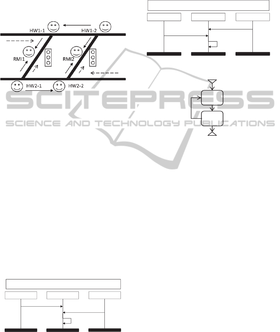
5.1.3 Example
Figure 1 illustrates the traffic situation, containing
two highways HW1 and HW2, and two ramps,
which are the exit ramps of HW2 and entrances of
HW1. The flow of vehicles in the highways and
ramps are depicted with dashed arrows. The inflow
and outflow of the ramps to HW1 and from HW2 is
controlled by ramp metering installations (RMI)
RMI1 and RMI2. When congestion starts to build up
on HW1 downstream of the second ramp, RMI2 will
detect this and reduce the inflow. Likewise, when
the exit ramp of HW2 starts to build up congestion,
RMI1 and RMI2 will take action to reduce
congestion. In order to have better performance and
ICAART2015-DoctoralConsortium
18
take better actions, RMI1 and RMI2 should be aware
of future congestion. Therefore, the system is
designed as a Multiagent System (MAS), which can
be considered as a subset of DSS, in which the
agents are capable of communicating to each other.
In this way, they can react in advance and solve the
congestion timelier.
Figure 1: Multiagent System for congestion control.
The system has two highway agents for each
highway and one RMI agent for each ramp. The
highway agents have the capability of developing an
image of the current traffic situation, depending on
their own estimation and incoming messages from
downstream agents. The arrows in Figure 1 indicate
the possible communications of each agent.
Highway agents can send “no problem”, “help-
urgent high”, and “help-urgent low” messages to
their neighbor agents and RMI agents. The RMI
agents can take actions “make the traffic light green”
or “make the traffic light red” based on the messages
they receive from highway agents.
Two scenarios of this system are described using
MSCs. These MSCs demonstrate a situation that the
first agents of highway one and two, HW1-1 and
HW2-1 respectively, requests urgent help from
RMI1. In the first MSC M1, the request of HW2-1 is
received sooner. Therefore, the RMI1 makes the
traffic light green. This is shown in Figure 2.
In MSC M2, illustrated in Figure 3, HW1-1
sends its help request sooner and RMI1 agent makes
the traffic light red.
Figure 2: MSC M1- Agent in HW2 requests high urgent
help.
The hMSC of these two MSCs is shown in
Figure
4
. The upside down triangle demonstrates the start
and the regular triangle exhibits the termination of
hMSC.
Figure 3: MSC M2- Agent in HW1 requests high urgent
help.
Figure 4: High level MSC of MAS congestion system.
5.2 Modeling Processes’ Interactions
We model the interaction of processes in each
into its corresponding interaction matrix
. An
interaction matrix is an square matrix of size
|| equal to the total number of processes in the
system. Two types of interaction matrices are
defined that are used for various communication
channels: Send Interaction Matrix and Receive
Interaction Matrix.
We define a send vector
,
,…,
for each process ∈ in an MSC . The elements
of
can have one of the following values:
1) ∃
∈,∃
∈ , ∃ ∈ ∃ ∈
!
.
2)∃
∈ ,
∈ ,
∈
∈
!
|
|
1
:
∪
.
3)
∈,∄∈,∄∈,∄∈
!
∅.
The send vector
consists of element where
||. The
is a set of sets {
,
,…,
.
The
is the set of all send events in which process
sends messages to another process
∈ in an
HW2-1
RMI1
Help-Urgent High
M1- Agent HW2-1 requests high urgent help
Green Light
HW1-1
Help-Urgent High
HW2-1
RMI1
Help-Urgent High
M2- Agent HW1-1 requests high urgent help
Red Light
HW1-1
Help-Urgent High
M 1
M 2
ANewApproachfortheDetectionofEmergentBehaviorsandImpliedScenariosinDistributedSoftwareSystems-
ExtractingCommunicationsfromScenarios
19

MSC . The three cases above, represent that
can have exactly one member (case 1), more than
one member (case 2), or be an empty set (case 3).
∪
.
A Send Interaction Matrix over is a
matrix that represents all communications in an
MSC that are of type “Sending”. The entries of
are
,
,…
where
∈ and
represents the
row in and
.
We define a receive vector
,
,…,
for each process ∈ in an MSC . The elements
of
can have one of the following values:
1) ∃
∈,∃
∈,∃∈∃∈
?
.
2) if
∃
q_i
∈
P,for some r_j
∈
R,and for some e_k
∈
R
and for some m_k
∈
M such that μ(e_k )=p?q_i
(m_k ) and |μ(e_k )|>1 then b_i is a set:
b_i=
∪
_j r_j
3)
∈,∄∈,∄∈,∄∈
?
∅.
The receive vector
consists of elements
where ||. The
is a set of sets
{
,
,…,
. The
is the set of all receive events
in which process receives messages from another
process
∈ in an MSC . The three cases
above, represent that
can have exactly one
member (case 1), more than one member (case 2), or
be an empty set (case 3).
∪
.
A Receive Interaction Matrix over is a
matrix that represents all communications in an
MSC that are of type “Receiving”. The entries of
are
,
,…
∈ and
represents the
row in and
. In FIFO communications, we have
for their corresponding MSC
, i.e. the
two matrices
and
are transpose of each
other. However, in other communication channels,
and
for their corresponding MSC
,
might be different based on the definitions of that
channel, and
.
We define a state vector
∪
,
,
,
,…,
for each process
∈ of an MSC where |
|. The state
vector
is the total order set of
in the MSC
with respect to its local visual order
:
∈
, ∃ ∈ , ∈ ,
!
∈ ,
?
For process we define
∪
with respect
to its global visual order
over
.
The state transition vector
,
,…,
for each process ∈ of an
MSC where |
|, represents the senders of
messages that cause a transition in states of process
in the MSC . Each action on the life time of
process in MSC is either !
or ?
for ∈. For ∈and ∀ ∈
:
!
?
We define
∪
as the total set of state
transitions for process ∈ over the set of
in
with respect to its global visual
order
.
The basic state diagram
,
is a
directed graph that represents the visual structure of
events
for each process ∈ of an MSC ,
where
,|∈
∈
is the set of nodes and
, , |, ∈
∈ is
the set of edges, where
∃ ∈
,
∈
!
?.
The state diagram
,
represents the
total set of states of process ∈ over the set of
MSCs .
∪
, where
∪
and
∪
.
We define a minimum state diagram
,
for process , where
⊆
and
⊆
. For
,
,
∈
, ∈
,
∈
, ∈,
,
∈
, and ∈
:
.
For
, ,
,
∈
,, ∈
,
, ,
,
∈ ,
,
∈
,
,
,
, and
,
,
:
1) if
.
2) if
and we define two edged
,
,
and
,
,
.
3) if
and we define two edged
,
,
and
,
,
.
In the minimum state diagram for each process, we
merge the vertices based on the states and the state
transition of that state. Therefore, if two vertices in
has the same vertex and edge, they are merged in
ICAART2015-DoctoralConsortium
20
one vertex in
(case 1). However, if any of the
states or state transitions (defined in the edges) are
different, two edges are displayed in the minimum
state diagram
. This indicates that the senders of
messages that change a state transition are
considered in merging the vertices. The latter
illustrates a branch in
(case 2 and 3).
Note that since the events
on process have a
local visual order
, the
relation is preserved in
the send, receive, and state vectors
,
, and
in the MSC . For the same reason,
,
,
and
follow the global visual order
in its high
level structure
.
5.3 Emergent Behaviors of
Asynchronous Concatenation
Emergent behaviors, also known as implied
scenarios, are referred to as unexpected behaviors of
processes (agents) during their execution, which
were not seen in their design. The word emergent
behavior is mostly used for the unexpected behavior
of one process without considering other processes
in the system. Implied scenarios are used for a
situation that an unexpected behavior occurs when
considering all processes in the system. In this case,
a new scenario is implied, and it is considered as
system level emergent behavior. Emergent behaviors
and implied scenarios both refer to unexpected
behaviors in the system; the only difference is that
the unexpected behavior is examined in component
or system level. Therefore, we may use these terms
interchangeably in this paper.
In asynchronous concatenation of MSCs in a
HMSC, the processes may proceed in next MSCs in
different times (Muscholl and Peled, 2005). Let
,
∈ be two MSCs from the set that
contains all MSCs of the system, and
precedes
in the HMSC . Consider processes , ∈
where
is the finite set of processes (agents) of
; and and have some actions in both
and
. In asynchronous concatenation of MSCs,
processes do not wait until all other processes
accomplish their actions in one MSC. Therefore,
while process is still involved in
, process
may proceed to perform its actions in
that we
refer to as issue I1.
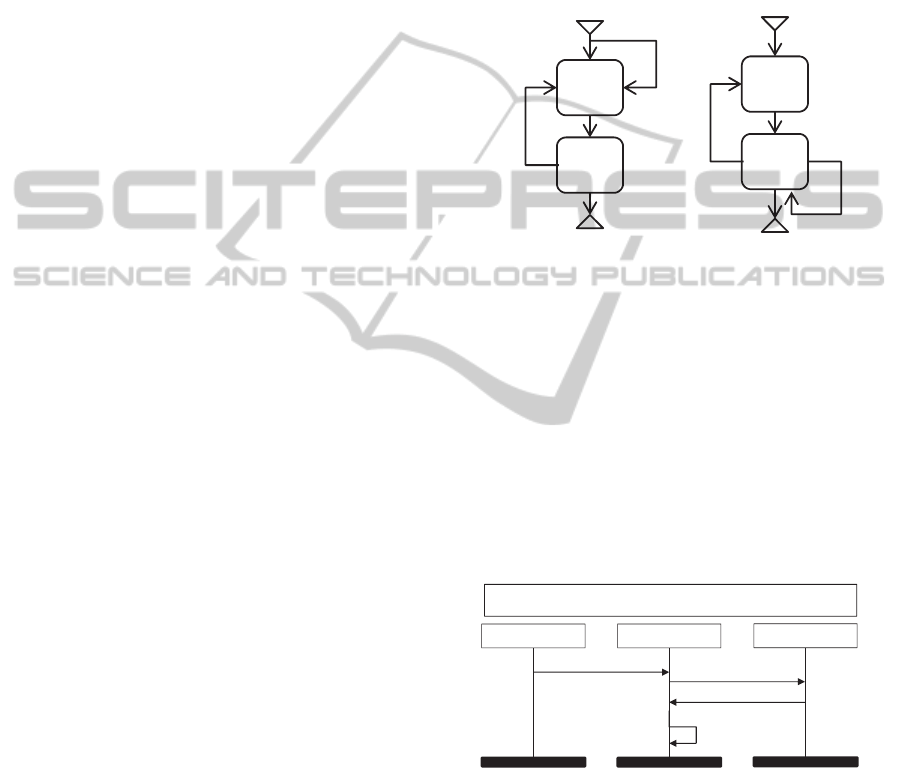
Consider the MAS system in the example. The
agent HW2-1 in MSC M1 can proceed to M2 and
send a request of “high urgent help” to agent RMI1;
while, HW1-1 is still proceeding its actions in M1.
This can result in a repetition in executing MSC M1.
Thus, an emergent behavior that is shown in Figure
5 (a) can happen. The same situation can occur for
HW1-1 in M2. Consequently, the MSC M2 is
repeated and emergent behavior of Figure 5 (b) can
arise.
The asynchronous concatenation of MSCs may
result in another issue I2. Let a third process ∈
that is involved in
,
∈ where it has
interactions with both processes and in
and
and it receives some messages from both
processes and .
Figure 5: Two emergent behaviors caused by issue I1.
In this case, there is no control over the receive
events on process line of when its senders are
different. This is referred to as a race condition in
the literature. The same situation can occur when
, , ∈
and process receives some messages
from process and in MSC ∈.
Let add another MSC to the MAS example that
is depicted in
Figure 6. In this MSC, M3, agent
HW2-1 send a low urgent help request to RMI1.
Therefore, RMI1 asks HW1-1 for its situation to
take the best action. Since the urgency of HW1-1 is
high, RMI1 makes the traffic light red.
Figure 6: MSC M3- Agent in HW2 requests low urgent
help.
An implied scenario that can occur is shown in
Figure 7. The agent HW2-1 can proceed to MSC M1
and send a high urgent request. Since there is no
control on the receiving messages of RMI1 that are
sent by different agents (HW2-1 and HW1-1), RMI1
may proceed to M1 and make the traffic lights
green.
M 1
M 2
M 1
M 2
(a)
(b)
HW2-1
RMI1
Help-Urgent Low
M3- Agent HW2-1 requests low urgent help
Red Light
HW1-1
Ask info
Help-Urgent High
ANewApproachfortheDetectionofEmergentBehaviorsandImpliedScenariosinDistributedSoftwareSystems-
ExtractingCommunicationsfromScenarios
21
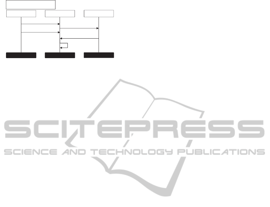
Figure 7: Implied scenario caused by issue I2.
5.3.1 Define Detection Rules for Issue I1
We define active and passive processes that are
processes that, whether or not, have control to start
an MSC, respectively. Since an active process sends
its first message in an MSC, the process does not
need to wait for an action that changes its state.
Therefore, an active process is the sender of its first
action that leads to a state transition for its first state.
However, this is not held for a passive process. A
passive process should wait for the sender of its
action to send it a message and changes its state.
Therefore, for a passive process, starting an MSC is
not in its control and depends on other processes.
The definitions for active and passive processes are:
Let processes , ∈ have some actions in
an ⊆ . We define process as an active
process in if for the first action of in its local
visual order
, the following condition is satisfied
in :
∃∈,∈|
!
Let processes , ∈ have some actions in
an ⊆ . We define process as a passive
process in if for the first action of in its local
visual order
, the following condition is satisfied
in :
∃∈,∈|
?
Let
⊆ as the set of MSCs in which a
process ∈ is an active process.
Rule R1: An active process ∈ can lead to issue
I1 in all MSCs ⊆
if there is no timing or
control over the MSCs. The reason is that process
has the control of starting an action in a new MSC in
.
Rule R2: Let process ∈ in hMSC
,,,,,∁,
,
, that has
structure
,
,
,
,∁
,
,
, be an active
process. Process can lead to issue I1 if one of the
following conditions holds:
1)
⊆
2)
∃ ∈
∁
⊆
3)
∃ ∈
∁
⊆
When the
, the structure of MSCs that an active
process ∈ follows, is different from the
structure of hMSC , which is defined as a global
view for all processes, it might lead to issue I1. The
first condition defines a situation in which the initial
MSC of
is different from the initial MSC in .
Therefore, process can start its high level
structure, without following the scenarios that the
whole system performs. The second condition, states
that the initial MSCs in
and are the same.
However, the termination MSC for is different. In
this situation, the active process starts its initial
MSC when the other processes start performing their
scenarios. However, it does not follow the same
scenarios that other processes are performing in
other iterations of the hMSC. Because the
termination nodes (final vertices) are different, can
start performing its high level structure
again,
while the other processes are performing actions in
the rest of MSCs in . The third condition, is a more
general condition in which process has different
initial and termination MSCs in
with initial and
termination MSCs in , respectively.
Rule R3: Issue I1 can occur when process has a
loop in its
structure, which is an internal loop in
hMSC ,,,,,∁,
,
. The loop in
is an internal loop when it does not include the
initial and termination vertices
and
. Process
can be either an active or a passive process.
When performs actions in an internal loop, it may
execute the loop more than other processes. The
termination MSCs are different in
and .
Therefore, can start performing
again, while
the other processes are continuing to perform their
actions in other MSCs in .
Rule R4: Consider an active or passive process
that has a loop in
,
,
,
,∁
,
,
from
to
. If this loop is an internal loop in hMSC
,,,,,∁,
,
, process can cause
issue I1.
The reason is similar to the reason of rule R3. The
final MSCs in
and are different. Therefore,
process can start executing its MSCs, while the
HW2-1
RMI1
Help-Urgent Low
Implied Scenario 3
Green Light
HW1-1
Ask info
Help-Urgent High
Help-Urgent High
ICAART2015-DoctoralConsortium
22

other processes are continuing their actions in other
MSCs.
5.3.2 Define Detection Rules for Issue I2
Suppose that processes ,, ∈ have interactions
with each other in an MSC . If process has at
least one receive message from each of the other
processes and , and there is no control over the
order of receive messages for process with respect
to its visual order
, a race condition can occur. In
this situation the visual order
in MSC is not
preserved.
Rule R5: Let
,…,
,…,
,…,
be the
receive vector of process in an MSC . The
elements
and
represent the set of events that
receives from processes and respectively. Let
,…,
,…,
,…,
be the new receive
vector for process , where the order of
and
has changed, compared to
. We have
∪
,
,
as the state vector of and
∪
,
,
as the new state vector
of process .
If
is not in the set of
∪
, then
process can cause issue I2 because of a change in
its receive orders:
∃,
∈;,
∈
;
,
∈∑
?
?
⊆
isanemergentbehaviorfor.
Rule R5 indicates that a change in the order of
receiving messages for process should be in the
events of process in other MSCs, or receiving of
such messages should be controlled, in order to
prevent an emergent behavior.
Rule R6: Let
,…,
,…,
,…,
be a
new receive vector for process , where the order of
and
has changed, compared to
and
∃
∈ such that
⊆
. Let
,
be the associated basic state diagram
for receive vector
and state vector
in .
Consider
,
as the associated
basic state diagram for receive vector
and state
vector
in
. We define
,
∈
as
the corresponding nodes in
, for the states of
process that receive messages from process and
, respectively. If
is not in
∪
, then
∪
,
,
is an emergent
behavior .
Rule R6 defines more restrictive criteria that a
process can have a behavior that leads to issue I2.
Other than the new receive vector in the states of
process , the state transition vectors should be
considered as well; to check whether or not a
process can lead to I2 and show an emergent
behavior.
A change in the order of states
and
,
resulted from communications with processes and
, in the receive states of process , creates a new
receive vector
. The
can exist in the state
vectors of in another MSC
. However, the
communicating processes associated to states
and
in
, may be different, namely, processes and
. Therefore, the two state vectors
and
,
are not considered as similar state vectors when
considering their associated state transitions;
because their communicating processes for these
two states (
and
) are different. In this situation,
although the state vectors in the two MSCs are the
same, process can still show an emergent
behavior, because of a difference in its state
transition vectors.
6 STAGE OF THE RESEARCH
Until now, the categories of emergent behaviors are
formalized. For each category, various conditions
and reasons that can lead to an implied scenario are
investigated, and some algorithms are devised. The
first parts of the methodology, including
transforming the designs into interaction matrices,
and detecting components with no emergent
behaviors are implemented. The current research
trend is focused on testing algorithms on large scale
systems, using communication of processes in Linux
clusters as the test bed.
ACKNOWLEDGEMENTS
This research is supported by a grant from Izaak
Walton Killam Memorial Scholarship, Alberta
Innovates Technology Futures and partially from
Natural Sciences and Engineering Research Council
of Canada.
REFERENCES
Aggarwal, C. C. (2011). An introduction to social network
data analytics (pp. 1-15). Springer US.
ANewApproachfortheDetectionofEmergentBehaviorsandImpliedScenariosinDistributedSoftwareSystems-
ExtractingCommunicationsfromScenarios
23

Alur, R., Etessami, K., & Yannakakis, M. (2005).
Realizability and verification of MSC graphs.
Theoretical Computer Science, 331(1), 97-114.
Bhateja, P., Gastin, P., Mukund, M., & Kumar, K. N.
(2007, January). Local testing of message sequence
charts is difficult. In Fundamentals of Computation
Theory (pp. 76-87). Springer Berlin Heidelberg.
Briand, L. C. (2010). Software Verification—A Scalable,
Model-Driven, Empirically Grounded Approach. In
Simula Research Laboratory (pp. 415-442). Springer
Berlin Heidelberg.
Chaki, S., Clarke, E., Grumberg, O., Ouaknine, J.,
Sharygina, N., Touili, T., & Veith, H. (2005, January).
State/event software verification for branching-time
specifications. In Integrated Formal Methods (pp. 53-
69). Springer Berlin Heidelberg.
Chakraborty, J., D’Souza, D., & Kumar, K. N. (2010).
Analysing message sequence graph specifications. In
Leveraging Applications of Formal Methods,
Verification, and Validation (pp. 549-563). Springer
Berlin Heidelberg.
Fard, F. H., & Far, B. H. (2013, August). Detecting
distributed software components that will not cause
emergent behavior in asynchronous communication
style. In Information Reuse and Integration (IRI), 2013
IEEE 14th International Conference on (pp. 201-208).
IEEE.
Holzmann, G. J., & Smith, M. H. (2002). An automated
verification method for distributed systems software
based on model extraction. Software Engineering,
IEEE Transactions on, 28(4), 364-377.
Iglesias, A. (2009). Software Verification and Validation
of Graphical Web Services in Digital 3D Worlds. In
Communication and Networking (pp. 293-300).
Springer Berlin Heidelberg.
ITU-T UNION, SERIES Z: languages and general
software aspects for telecommunication systems -
Formal description techniques (FDT) – Message
Sequence Chart, 2004, ITU-T Recommendation
Z.120. p. 136.
Krüger, I. H. (2000). Distributed system design with
message sequence charts(Doctoral dissertation,
Technische Universität München,
Universitätsbibliothek).
Letier, E., Kramer, J., Magee, J., & Uchitel, S. (2005,
May). Monitoring and control in scenario-based
requirements analysis. In Proceedings of the 27th
international conference on Software engineering (pp.
382-391). ACM.
Mousavi, A. (2009). Inference of emergent behaviours of
scenario-based specifications (Doctoral dissertation,
UNIVERSITY OF CALGARY).
Muscholl, A., & Peled, D. (2005). Deciding properties of
message sequence charts. In Scenarios: Models,
Transformations and Tools (pp. 43-65). Springer
Berlin Heidelberg.
Song, I. G., Jeon, S. U., Han, A. R., & Bae, D. H. (2011).
An approach to identifying causes of implied scenarios
using unenforceable orders. Information and Software
Technology, 53(6), 666-681.
Uchitel, S. (2003). Incremental elaboration of scenario-
based specifications and behaviour models using
implied scenarios (Doctoral dissertation, Imperial
College London (University of London)).
Uchitel, S. (2009). Partial Behaviour Modelling:
Foundations for Incremental and Iterative Model-
Based Software Engineering. In Formal Methods:
Foundations and Applications (pp. 17-22). Springer
Berlin Heidelberg.
Uchitel, S., Kramer, J., & Magee, J. (2002, November).
Negative scenarios for implied scenario elicitation. In
Proceedings of the 10th ACM SIGSOFT symposium
on Foundations of software engineering (pp. 109-118).
ACM.
ICAART2015-DoctoralConsortium
24
