Modeling and 2D/3D-visualization of Geomagnetic Field and

Its Variations Parameters

Andrei V. Vorobev and Gulnara R. Shakirova

Department of Computer Science and Robotics, Ufa State Aviation Technical University, K. Marx St., Ufa, Russia

gimslab@yandex.ru

Keywords: Geoinformation Systems, Geomagnetic Field, Geomagnetic Variations, 2D/3D-visualization.

Abstract: In the modern World, specialists in biology, medicine, geophysics, geology, technics and many other

sciences pay great attention to correlation between external geomagnetic variations (GVM) with

possibilities of objects and systems existence and evolution. Well-known scientific publications give a quite

wide review of approaches to estimation of weak magnetic fields parameters, creation of magnetometric

information measurement systems on their base and definition of their metrological characteristics. But

today due to the recently formulated relevance of geomagnetic field (GMF) and its variations parameters

monitoring there is no unified and effective approach to development of geoinformation magnetometric

systems. In spite of the wide variety of specialized geoinformation systems (GIS) there are no advanced

hard- and software, which provide a calculation, geospatial connection, visualization and analysis of GMF

and its variations parameters calculation results. It is important to mention, that due to low-efficiency,

limited functionality and incorrect work of the known solutions the topicality, scientific and applied interest

to such a solution development continuously increases.

1 INTRODUCTION

In the modern World, specialists in many spheres

pay great attention to correlation between external

geomagnetic variations (GVM) with possibilities of

existence and evolution of objects and systems. This

interest is based on idea, that some components of

GMV or their combinations can influence on

biological, technical, geological and other objects

and systems in common and on human in particular.

As a result, the distorted normal conditions of

existence force these objects and systems to either

adapt to the changes of magnetic state (via

deformation, mutation, etc.) or keep existing there in

stressed (unstable) mode (Chizhevskii, 1976);

(Vernadsky, 2004).

Today monitoring, registration, visualization,

analysis, forecast and identification of GMV is a

relevant sophisticated fundamental scientific

problem with strong applied character.

In contemporary world the problem of

monitoring of geomagnetic field (GMF) and its

variations parameters is partially solved by a number

of magnetic observatories [Vorobev, 2012]. The

magnetic observatory is a scientific organization,

which is specialized on parametric and necessary for

them astronomical observations of the Earth’s

magnetosphere. The registered information about

magnetic field and ionosphere state is regularly sent

to the International centers in Russia, USA,

Denmark and Japan. In these centers the information

is registered, analyzed and partially available to the

broader audience with some delay. Today there are

about 100 geomagnetic observatories, and one third

of them are in Europe.

In spite of the wide variety of specialized

geoinformation systems (GIS) there are no advanced

hard- and software, which provide a calculation,

geospatial connection, visualization and analysis of

GMF and its variations parameters calculation

results.

An example of modern programming solution

with GIS features is the service, which is provided

by NOAA (National Oceanic and Atmospheric

Administration) and available at

http://www.ngdc.noaa.gov/geomag-web. However

the calculation results are out of limits of

permissible errors. It is takes no much time to ensure

about incorrect work of some tools, absence of

visualization tools and multilingual support, bad

geolocation and non-informative interface.

It is important to mention, that due to low-

V. Vorobev A. and R. Shakirova G..

Modeling and 2D/3D-visualization of Geomagnetic Field and Its Variations Parameters.

DOI: 10.5220/0005348200450053

In Proceedings of the 1st International Conference on Geographical Information Systems Theory, Applications and Management (GISTAM-2015), pages

45-53

ISBN: 978-989-758-099-4

 2015 SCITEPRESS (Science and Technology Publications, Lda.)

efficiency, limited functionality and incorrect work

of the known solutions the topicality, scientific and

applied interest to such a solution development

continuously increases.

2 MATHEMATICAL MODELING

OF GEOMAGNETIC FIELD

AND ITS VARIATIONS

The full vector of the Earth’s magnetic field

intensity in any geographical point with

spatiotemporal coordinates is defined as follows:

= B

+ B

where B

is an intensity vector of GMF of

intraterrestrial sources; B

is a regular component of

intensity vector of GMF of magnetosphere currents,

which is calculated in solar-magnetosphere

coordinate system; B

is a GMF intensity vector

component with technogenic origin.

Normal (undisturbed) GMF is supposed as a

value of B

vector with excluding a component,

which is caused by rocks magnetic properties

(including magnetic anomalies). So this component

is excluded as a geomagnetic variation:

= B

– ΔB '

where B

is undisturbed GMF intensity in the point

with spatiotemporal coordinates; ΔB'

is component

of intraterrestrial sources GMF, which represents

magnetic properties of the rocks.

Solving the problem of B

parameters analytical

estimation, it is helpful to represent the main field

model by spherical harmonic series, depending on

geographical coordinates.

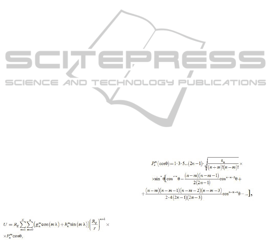
The scalar potential of intraterrestrial sources

GMF induction U [nT·km] in the point with

spherical coordinates r, θ, λ is defined by the

expression (1).

(1)

where r is a distance from the Earth’s center to

observation point (geocentric distance), [km]; λ is a

longitude from Greenwich meridian, [degrees]; θ is a

polar angle (collatitude, θ = (π/2)-φ’, [degrees],

where φ’ is a latitude in spherical coordinates,

[degrees]); R

is an average radius of the Earth,

= 6371.03, [km]; g

(t), h

(t) are spherical

harmonic coefficients, [nT], which depend on time;

are Schmidt normalized associated Legendre

functions of degree n and order m.

In geophysical literature the expression (1) is

widely known as a Gaussian and generally

recognized as an international standard for

undisturbed state of GMF.

The amount of performed spherical harmonic

analysis is significant. However a problem of

spherical harmonic optimal length of still acute.

Thus, the analyses with great amount of elements

prove Gauss hypothesis about convergence of

spherical harmonic, which represents a geomagnetic

potential. As usual in spherical harmonic analyses

the harmonics are limited by 8–10 elements. But for

sufficiently homogeneous and highly accurate data

(for example, as like as in satellite imaging) the

harmonics series can be extended up to 12 and 13

harmonics. Coefficients of harmonics with higher

orders by their values are compared with or less than

error of coefficients definition.

Due to the main field temporal variations the

coefficients of harmonic series (spherical harmonic

coefficients) are periodically (once in 5 years)

recalculated with the new experimental data.

The main field changes for one year (or secular

variation) are also represented by spherical

harmonics series, which are available at

http://www.ngdc.noaa.gov/IAGA/vmod/igrf11coeffs

.txt.

Schmidt normalized associated Legendre

functions P

from expression (1) in general can be

defined as an orthogonal polynomial, which is

represented as follows (2).

(2)

where ε

is a normalization factor (ε

= 2 for m ≥ 1

and ε

= 1 for m = 0); n is a degree of spherical

harmonics; m is an order of spherical harmonics.

3 GEOMAGNETIC

PSEUDOSTORM EFFECT

Here it is supposed to enter the term geomagnetic

pseudostorm (GMPS), which is intended to represent

real GMF influence on the object in conditions of its

non-zero speed and undisturbed GMF anisotropy

(Vorobev and Shakirova, 2014). Let us describe

some main parameters of GMPS effect (Vorobev,

GISTAM2015-1stInternationalConferenceonGeographicalInformationSystemsTheory,ApplicationsandManagement

2013).

GMPS range is a difference between maximal

and minimal values of GMF induction in area of the

object, which is moving in anisotropic magnetic

field during the time period or at the distance:

GMPS

= B

0 max

– B

0 min

, (3)

where B

0 max

and B

0 min

are maximal and minimal

values of GMF induction, [nT] in area of the object,

which is moving in anisotropic magnetic field.

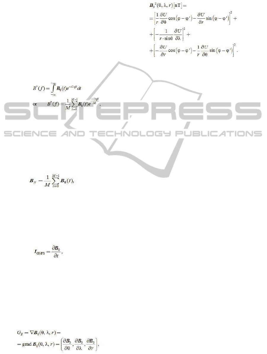
GMPS frequency spectrum is a function of

distribution of GMPS amplitude spectrum in

frequency area for continuous and discrete variants,

which is defined by the following expressions:

(4)

where B* is a GMPS frequency spectrum; B

is a

value of GMF induction in the point with

spatiotemporal coordinates; M is a quantity of

registered values with constant discretization step by

time.

Constant component of GMPS is a vector of

harmonics superposition vertical shift, which

represent GMPS frequency spectrum:

(5)

where M is a quantity of registered values with the

discretization step.

GMPS intensity is a physical quantity, which is

numerically equal to the speed of undisturbed GMF

characteristic change in time relatively to the frame

of reference, which is connected to the moving

object and depends on the object speed:

(6)

where I

GMPS

is GMPS intensity, [nT/s];

GMPS potentiality (geomagnetic induction

gradient) is a vector, which is oriented in three-

dimensional space and points to the direction of the

fastest increase of undisturbed GMF induction

absolute value. The vector by its absolute value is

equal to the increase speed of B

in the geographical

direction, [nT/rad; nT/rad; nT/km] and depends on

the object position.

(7)

where B

is an induction (intensity) of GMF in the

point with spatiotemporal coordinates:

(8)

So the analysis of GMF induction gradient

distribution allows defining an area of possible

GMPS maximal intensity of in the geographical

region. So, the parameter G

must be taken into

account in developing aerospace navigation maps

and flight paths (Milovzorov and Vorobev, 2013).

Next to study the GMPS effect there is an

example of the flight route AA-973 of «American

Airlines» from New York (JFK) to Rio de Janeiro

(RIO). The flight path is represented as an array of

spatial coordinates, which describe the airplane

position, taken during flight in equal time intervals.

The array allows calculating GMF parameters for

each set of spatial coordinates.

The results of amplitude and frequency analysis

of flight data and parameters of GMF are

represented on Figure 1. Here are some special

points (Figure 1, a): t1-t2 – takeoff time; t2-t4 –

flight on cruise speed at the altitude of 11033 m; t4-

t5 – landing time; t3 – passing the equator.

4 VISUALIZATION OF

GEOMAGNETIC FIELD

PARAMETERS

An effective solution for complicated problem of

modeling and visualization of GMF and its

variations parameters is a key to understand the

principles of GMF parameters distribution on the

Earth’s surface, its subsoil and in circumterrestrial

space.

Modern information technologies provide wide

variety of tools for both in mathematical modeling

and computer graphics. However a problem of

parametric GMF and its variations model is still not

solved.

So, one of the effective approaches to solve the

problem is a functionality of modern GIS, which

special and applicative implement supposes rather

suitable result.

Modelingand2D/3D-visualizationofGeomagneticFieldandItsVariationsParameters

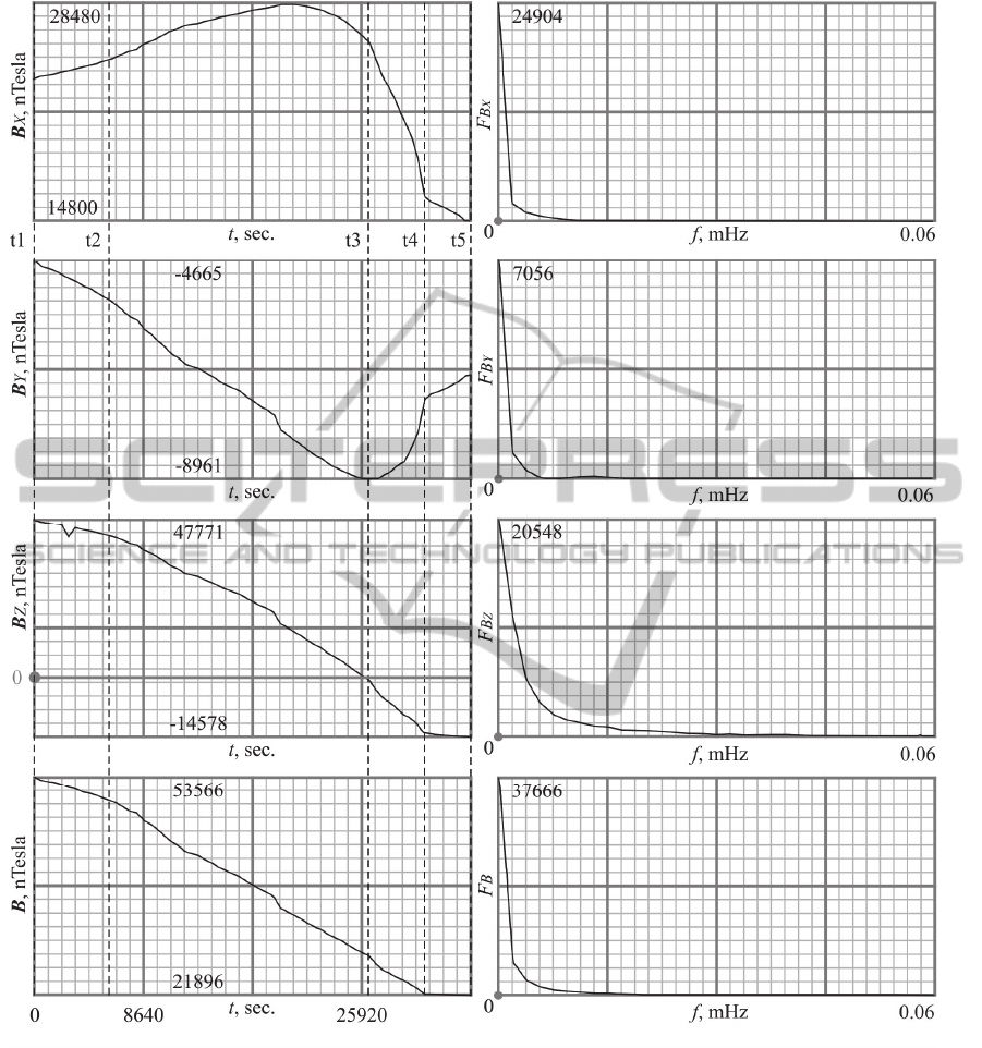
a b

Figure 1: Experimental data analysis results.

Three-dimensional representation of research

(calculation) results is one of the key aspects in

solution of visualization problems of both geospatial

data and GMF parameters. It is obvious, that in this

case GIS provides much more information. And it is

even more important due to the dynamic properties

and multilevel scale ability.

As a result of our research there was developed

the special GIS, which is based on modern web

technologies and provides great functionality for

both calculation of GMF, its variations and

anomalies parameters calculation and visualization

of the results distribution in terrestrial and

circumterrestrial space. The developed Web GIS

combines the development principles and

possibilities of distributed client-server web

application and geoinformation systems. This GIS

provides the complex calculation and visualization

GISTAM2015-1stInternationalConferenceonGeographicalInformationSystemsTheory,ApplicationsandManagement

of GMF parameters with any scale (The service is

available at http://gimslab.url.ph). The main

modules of the suggested GIS are Web GIS "GIMS-

Calculator" and "GIMS-Pseudostorm Analyzer"

(Vorobev and Shakirova, 2013); (Vorobev and

Shakirova, 2014).

The main functionality of Web GIS "GIMS-

calculator" provides effective and reliable

calculation and analysis of parameters of normal

(undisturbed) GMF by the spatiotemporal

coordinates with error value no more than 0.1%.

To provide the ergonomics of software the

"GIMS-calculator" window is logically divided into

two functional areas (panels). Left panel (Figure 2)

is supposed for loading and rendering the Earth’s

surface maps fragments in either scheme or photo.

Right panel is supposed for representing the input

parameters / initial conditions, calculation results

and "GIMS-calculator" functionality control. (The

initial conditions are defined as spatiotemporal

default coordinates: 54.7249° N, 55.9425° E,

0.172 km amsl).

For the appropriate tasks a user defines the

spatiotemporal coordinates of the Earth’s surface

point. These coordinates can be described by one of

the following ways:

 pick the point on the map (coordinates set up and

geocoding are performed automatically);

 latitude, longitude, altitude values input to the

appropriate input fields in the right panel of

application "GIMS-calculator";

 automatic detection of the user position on the

basis of the computer (or mobile device)

geolocation by IP address.

An important feature of "GIMS-calculator" is data

representation in one of the two formats: DD

(decimal degrees) and DMS (degrees – minutes –

seconds). Depending on the chosen format a user

gets the appropriate input mask. Also the application

supposes the automatic transformation of coordinate

systems via checking the appropriate radio button.

On the basis of latitude and longitude input

values "GIMS-calculator" automatically calculates

the altitude and represents the result in International

System of Units or Imperial and US customary

measurement systems. As in previous case, the

direct and indirect transformations are available.

User-defined spatiotemporal coordinates put the

center of the map visible fragment relatively to the

geographical point, which is defined by them. The

point is outline by the marker with geolocation

results.

"GIMS-calculator" special feature is a function

of detecting the current location. Geospatial

coordinates of user location are defined by IP

address of device, which is used for accessing the

Internet. This possibility allows the user to get the

point without its searching on the map or filling the

appropriate input fields. This feature increases its

efficiency and speed of the research.

The results of GMF parameters complex

calculation are represented in International System

of Units. This allows analyzing the data without any

preliminary calculations.

To extend the functionality of the developed

Web GIS "GIMS-calculator" there were

programmed an option of generating electronic

report about the research results with file or printer

form and a possibility of three-dimensional

modeling.

On the logical and programming levels the web

application is a set of complex procedures, which

provide the realization of geospatial data

visualization and analysis of GMF parameters in the

point with spatiotemporal coordinates.

With the lower abstraction the web application is

a special case of web page, which is developed

according three-tier client-server architecture. The

visible and adapted to the user (after rendering)

markup of the page is realized via W3C-

standardized markup language HTML (specifically,

its XML-type modification XHTML).

The page design is performed in traditional table

style: each region of the page is the table cell of

various levels. However, the table-like layout of the

page is not the only design solution here: there is

also block-type layout via HTML-elements div,

which logically structure the page by its semantics.

For example, one block HTML-element stands for

the region with map, another – for the region with

spatiotemporal coordinates, and the last – for the

region with GMF parameters calculation results.

Modelingand2D/3D-visualizationofGeomagneticFieldandItsVariationsParameters

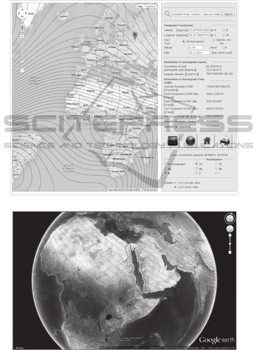
Figure 2: Detailed (regional level) interface of "GIMS-calculator".

Figure 3: Integration of GMF parameters research results with technologies KML and Google Earth.

GISTAM2015-1stInternationalConferenceonGeographicalInformationSystemsTheory,ApplicationsandManagement

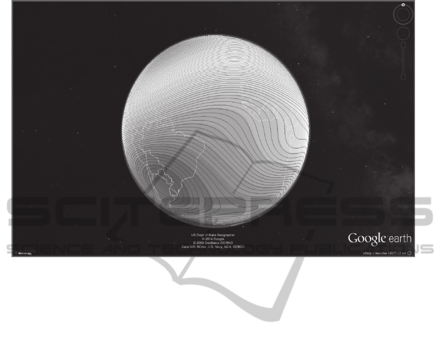
Figure 4: Fragment of intraterrestrial sources GMF induction full vector distribution on the Earth’s surface three-

dimensional model.

The technology of rendering the data by

spatiotemporal coordinates is based on the principle

of drawing geographical maps via mapping services

and specifically – one of the most functional and

popular Google Maps (Svennerberg, 2010); (Mapes,

2008); (Hu and Dai, 2013).

One of the most effective solutions for GMF

parameters calculation and research results

visualization is an approach, which is based on

three-dimensional web modeling. Usually this

approach supposes information representation on

two levels: geographical and attributive.

Geographical description of geospatial data supposes

three-dimensional visualization of the Earth’s

surface with variable zoom and detail parameters.

And the attributive component of the data is a set of

numerical values, which correspond to GMF

parameters values for spatial coordinates with an

appropriate step.

Today a problem of geographical and attributive

spatial data three-dimensional visualization is

usually solved via web applications of special type,

which are known as virtual globes. It is important to

mention, that virtual globes technology is based on

the Earth’s surface representation as a sphere with

applied graphical layers.

An important feature of the technology is its

availability in both user (client) and programming

services. A user version of virtual globe is oriented

on creation or load of applied layers, their

visualization and analysis of the synthesized model.

Typically the layers of the virtual globe are

represented as an optionally using markup (for

example, KML or KMZ archive).

Today one of the most popular versions of virtual

globes is Google Earth technology, which combines

the possibilities of desktop and web applications

(Haklay, 2008); (Dalton, 2013). This technology

provides a wide variety of functions for visualization

and multiaspect analysis of the Earth’s surface.

GMF analysis via client-type virtual globe is

concerned with rendering the thematic layer and

legend, which represent the calculated parameters in

the Earth’s surface points. In turn, this task can be

solved by a majority of known GIS (for example,

ArcGIS 10.2).

Geoformat of markup allows integrating

spherical representation of the surface with the map,

which is developed with GIS tools in some format,

for example, KML (Keyhole Markup Language is

one of the most popular formats of geodata

representation, which is supposed as XML-oriented

description of three-dimensional model of the

Earth’s surface and the objects on it. The description

on KML is a set of geographical and attributive

data). As a result there is a spherical representation

Modelingand2D/3D-visualizationofGeomagneticFieldandItsVariationsParameters

of the Earth’s surface with spatial data about GMF

parameters.

Virtual globes integration with applications is

provided by special API, which is a set of

programming functions for creation, visualization

and manipulation of three-dimensional spatial data.

Programming interface is used by an application

as a set of local or remote functions. These functions

can be used with the special possibilities of

interpreter, which is already used or additionally

loaded on user computer.

Typical example of virtual globes programming

interface is a plug-in Google Earth and its API on

the basis of JavaScript (Flanagan, 2011).

Functionality of the API provides the Earth’s three-

dimensional model inbuilt into the web application

and extend it with markers, infowindows, analytical

functions, etc.

So, Figure 3 demonstrates an example of

integrating the GMF parameters research results

with KML and Google Earth technologies. The

GMF induction full vector is visualized as a set of

isolines.

Isoloines are represented in special KML layer,

which in necessity can be overlaid on any other layer

(for example, data about seismic, volcanic activities,

medical statistics, geological maps, etc.). It provides

an effective tool for complex analysis of various

parameters, correlation and principles definition.

Numerical value of the parameter (physical value),

which is distributed along the one isoline, is

available via picking the appropriate line with mouse

cursor.

Various methods of visual data representation

(color outlining, gradient, etc.) increase the model

informativeness to maximum (Figure 4). Active

layers (country borders, cities, rivers, etc.) managing

keeps the key points of the model with decreasing

the probability of possible error.

So, GMF and its variations models, which are

represented and described here, meet the

requirements of specialists in various areas. They

effectively provide formatting and structuring the

data about the Earth’s magnetosphere parameters

and their further analysis.

5 CONCLUSIONS

 GMF is a complex structured natural matter with

ambiguous field characteristics, which is

distributed in the Earth (and near-Earth) space

and interacts with both astronomical objects and

objects / processes on the Earth’s surface, subsoil

and in near-Earth space. Research and analysis of

natural events, which cause GMV, allowed to

define the most probable amplitude and

frequency range for GMV:

ΔB [3·10-9–20·10-6] T; f [0–8] Hz.

 Approaches, criteria and classification features

for GIS description and classification on various

abstraction levels are defined, described and

scientifically proved.

 Analysis of modern tendencies of GIS evolution

proved, that the optimal direction of further

research is concerned with development,

realization and implementation of special GIS.

The special GIS is based on modern web

technologies and provides great functionality for

both calculation of GMF, its variations and

anomalies parameters calculation and

visualization of the results distribution in

terrestrial and circumterrestrial space.

 Web GIS "GIMS-Calculator" и "GIMS-

Pseudostorm Analyzer" are developed and

realized. These solutions provide the complex

calculation, analysis and visualization of GMF

and its variations parameters. According to

previous chapters visual models of the main

GMF parameters distribution on the Earth’s

surface are developed and represented (for 2014

year). These parameters are: north component of

GMF induction vector; vertical component of

GMF induction vector; magnetic declination and

dip; scalar potential of GMF induction vector.

 On the basis of web technologies in general and

technologies of modern virtual globes in

particular there were developed and described

innovative three-dimensional dynamic models of

GMF parameters distribution in circumterrestrial

space. The model provides multilayer

visualization as an effective tool for complex

analysis of various geophysical parameters and

definition of the appropriate correlations and

principles.

ACKNOWLEDGEMENTS

The reported study was supported by RFBR,

research projects No. 14-07-00260-a, 14-07-31344-

mol-a, 15-17-20002-d_s, 15-07-02731_a, and the

grant of President of Russian Federation for the

young scientists support MK-5340.2015.9.

GISTAM2015-1stInternationalConferenceonGeographicalInformationSystemsTheory,ApplicationsandManagement

REFERENCES

Vorobev, A. V., Shakirova, G. R., 2014. Pseudostorm

effect: computer modelling, calculation and

experiment analyzes. In Proceedings of the 14th

SGEM GeoConference on Informatics, Geoinformatics

and Remote Sensing, Vol. 1, p. 745–751 (Scopus,

DOI: 10.5593/sgem2014B21)

Vorobev, A. V., 2012. Digital geomagnetic observatories

development. LAP Lambert Academic Publishing G

mbh & Co. KG, Berlin.

Chizhevskii, A. L., 1976. Earth echo of sun storms.

Moscow: Mysl.

Vernadsky, V. I., 2004. The biosphere and the noosphere.

Moscow: Iris Press.

Vorobev, A. V., 2013. Geomagnetic pseudostorm effect

modeling and research. In Geoinformatics, No. 1,

pp. 29-36.

Milovzorov, G. V., Vorobev, A. V., Milovzorov, D. G.,

2013. Geomagnetic pseudostorm parameters

description methodics. In Vestnik IzhGTU, No. 1,

pp. 103-107.

Vorobev, A. V., Shakirova, G. R., 2013. Automated

analysis of undisturbed geomagnetic field on the basis

of cartographic web services technology. In Vestnik of

Ufa State Aviation Technical University. Vol. 17,

No. 5(58). pp. 177-187.

Dalton, C. M., 2013. Sovereigns, Spooks, and Hackers: An

Early History of Google Geo Services and Map

Mashups. In Cartographica, No. 48, pp. 261-274.

Haklay, M., Singleton, A. and Parker, C., 2008. Web

Mapping 2.0: The Neogeography of the Geo Web. In

Geography Compass, No. 2, pp. 2011-2039.

Mapes, J., 2008. Mapping for the Masses: Google

Mapping Tools. In Visual Studies, No. 23, pp. 78-84.

Svennerberg, G., 2010. Beginning Google Maps API 3.

Apress & Springer, New York.

Flanagan, D., 2011. JavaScript: The Definitive Guide. 6

Edition, O’Reilly Media Inc., Sebastopol.

Hu, S.F. Dai, T., 2013. Online Map Application

Development Using Google Maps API, SQL Database,

and ASP.NET. In International Journal of Information

and Communication Technology Research, No. 3,

pp. 102-111.

Modelingand2D/3D-visualizationofGeomagneticFieldandItsVariationsParameters