OpenGLSL-based Raycasting
Comparison of Execution Durations of Multi-pass vs. Single-pass Technique
Stefan Maas and Heinrich Martin Overhoff
Medical Engineering Laboratory, Westfälische Hochschule, Neidenburger Straße 43, Gelsenkirchen, Germany
Keywords: OpenGLSL, Raycasting, GPU, Volume Rendering.
Abstract: Real time volume rendering of medical datasets using raycasting on graphics processing units (GPUs) is a
common technique. Since more than 10 years there are two established approaches for realizing GPU ray
casting: multi-pass (Kruger and Westermann, 2003) and single-pass (Röttger, et al., 2003). But the required
parameters to choose the optimal raycasting technique for a given application are still unknown. To solve
this issue both raycasting techniques were implemented for different raycasting types using OpenGLSL
vertex and fragment shaders. The different techniques and types were compared regarding execution times.
The results of this comparison show that there is no technique faster in general. The higher the
computational load the more indicates the use of the multi-pass technique.
1 INTRODUCTION
In the last few years GPUs have become the most
important means for direct volume rendering (DVR).
Raycasting is the state of the art technique for
realizing DVR on GPUs (Marques, et al., 2009),
(Mensmann, et al., 2010). There are two basic
approaches for realizing GPU raycasting: multi-pass
and single-pass. These approaches differ in how they
calculate the ray marching direction vectors.
The multi-pass approach, as implemented by
(Kruger & Westermann, 2003) works as follows
when using OpenGLSL vertex and fragment
shaders:
A volume dataset is stored in the graphics
memory as a 3-D texture. 3-D textures are indexed
with texture coordinates
(x_coord, y_coord, z_coord) ∈[0.0, 1.0].
(1)
The next steps are:
Pass 1: The front facing faces of the volume
bounding box are rendered to a texture with 3-D
texture coordinates (1) as RGB-encoded color
values. These coordinates are the ray start positions
for the raycasting.
Pass 2: The back facing faces of the volume
bounding box are rendered to another texture with
3-D texture coordinates (1) as encoded color values.
These coordinates are the ray exit positions for the
raycasting. Based on the coordinate information of
passes 1 and 2, the ray directions can be calculated.
The directions are rendered as color to another 3-D
texture for use in the last pass.
Pass 3: The raycasting is performed by a
fragment shader casting each ray along the
calculated direction through the volume using a
given step size.
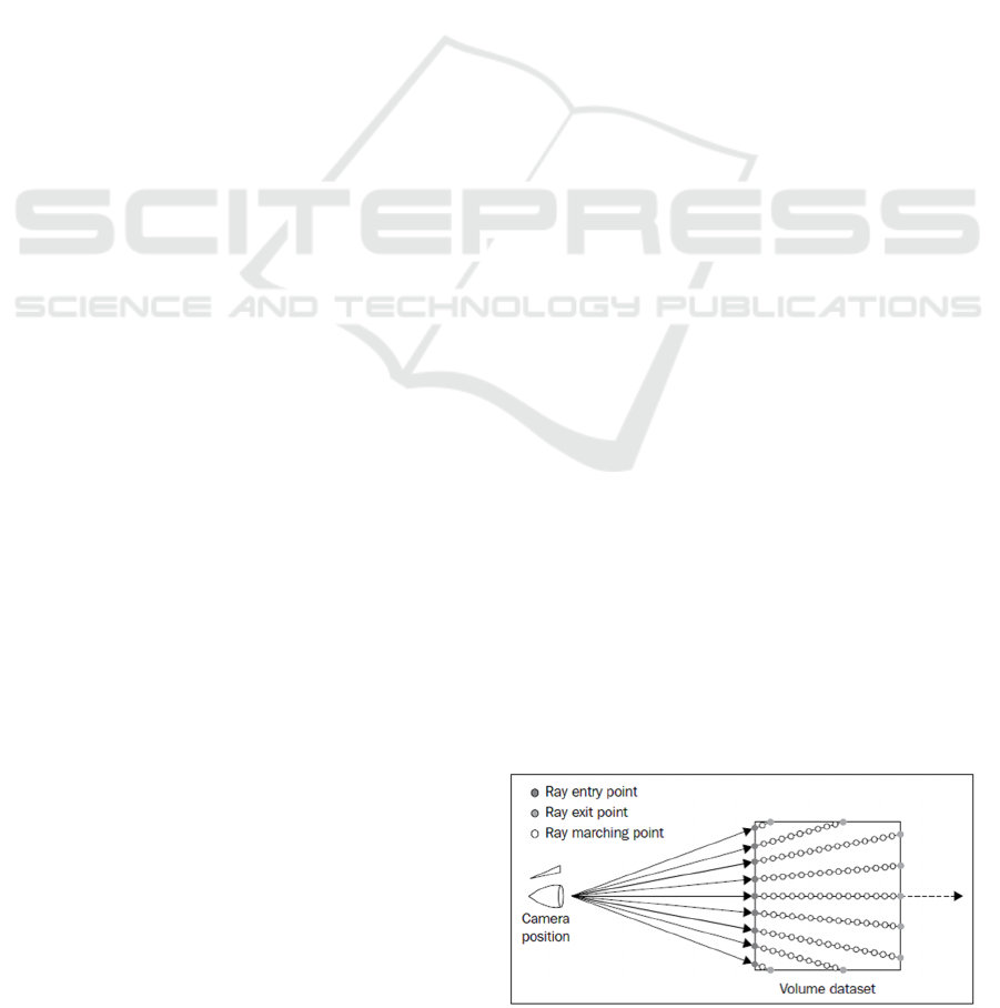
The single-pass approach (Röttger, et al., 2003)
uses only a fragment shader to calculate the ray
entry and exit points and performs the raycasting
(figure 1). The ray directions are calculated by
subtracting the vertex position from the camera
position. The ray entry positions are the positions of
the front vertices. From here the raycasting performs
like in pass 3 of multi-pass raycasting until the ray
exits the volume.
Figure 1: Single-pass raycasting (Movania, 2013).
The advantage of single-pass raycasting is its
simplicity. Due to the reduction of textures and
307
Maas S. and Overhoff H..
OpenGLSL-based Raycasting - Comparison of Execution Durations of Multi-pass vs. Single-pass Technique.
DOI: 10.5220/0005344703070310
In Proceedings of the 6th International Conference on Information Visualization Theory and Applications (IVAPP-2015), pages 307-310
ISBN: 978-989-758-088-8
Copyright
c
2015 SCITEPRESS (Science and Technology Publications, Lda.)
saving of many OpenGL calls regarding the volume
bounding box creation, it should be faster than
multi-pass raycasting. The disadvantage is the full
computational load on the fragment shader
(Venkataraman, 2009) which could slow down the
raycasting.
Different optimization techniques can be
implemented to lower execution times (ETs). One of
the most common techniques is the “Early Ray
Termination” (ERT) (Matsui, et al., 2005). It was
implemented because of its high potential of
lowering the ET while being easy to realize in
OpenGLSL.
Currently the required parameters to choose the
optimal raycasting technique for a given application
are unknown. The comparison reported here shall be
a first contribution to clarify this issue.
2 MATERIALS AND METHODS
Both raycasting techniques were implemented using
C# and OpenGLSL 4.3 (with OpenGL4Net
(Vanecek, 2014)). The engaged hardware consists of
a notebook (Windows 7 SP1, Intel Core i5-4200M
CPU, 2.5 GHz, 16 GB RAM) with an NVIDIA
Quadro K3100M (driver version 312.32) graphics
card. The raycasting is performed using an
ultrasound image volume with 512×378×222
grayscale values (8bit, unsigned integer), a voxel
spacing of 0.42 mm×0.39 mm×0.63 mm and a
viewport size of 1440×900.
For the comparison three different raycasting
types were implemented with and without ERT.
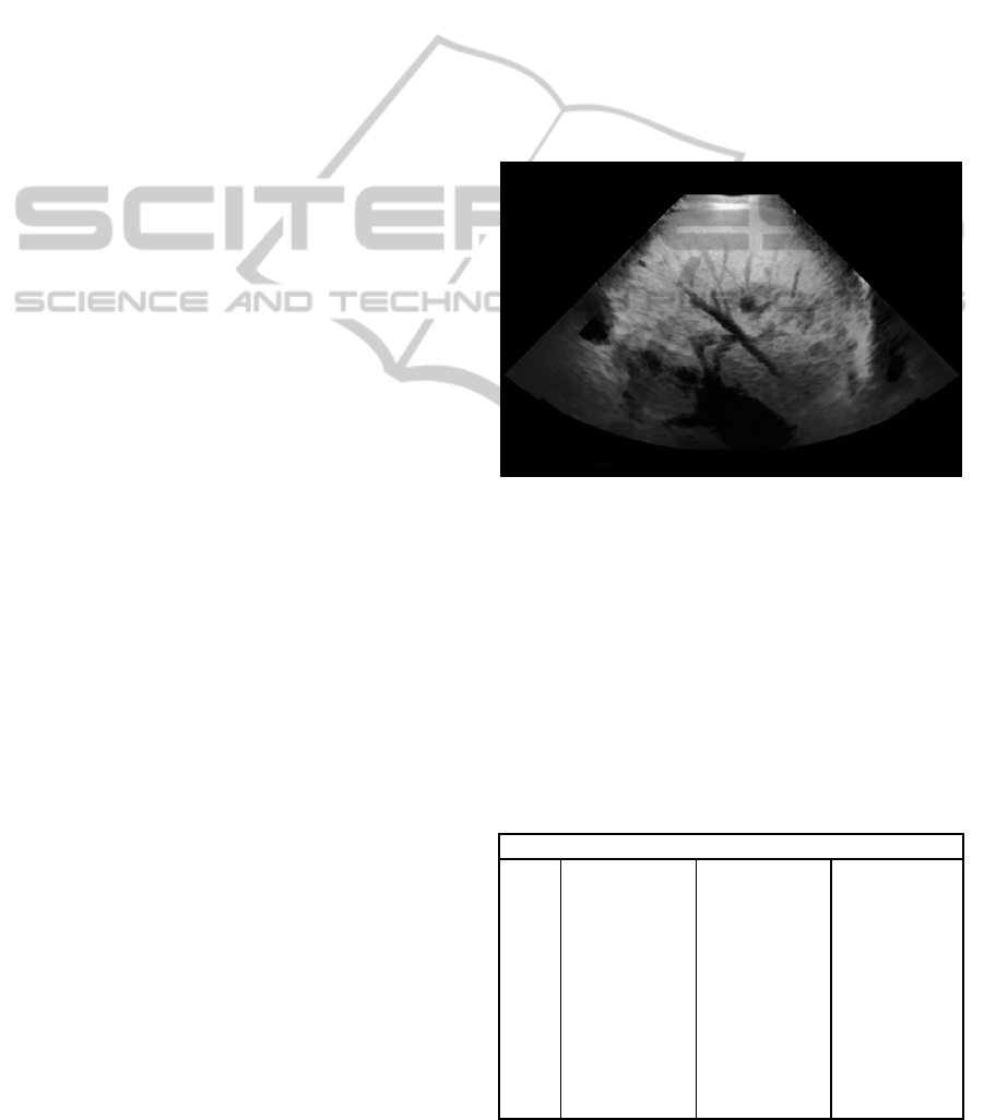
1. “Minimum Intensity Projection” (MINIP)
(Radiopaedia.org, 2014) - a simple rendering
technique to visualize e.g. liver vessels in
ultrasound volumes (figure 2) – as a technique
with low computing time.
2. Alpha Blending (Porter & Duff, 1984) as a
technique with medium computing time.
3. Gradient Calculation using the left and right
neighbor of each pixel along the ray as a
technique with high computing time due to many
texture fetches.
To measure the ET of the raycasting techniques the
following steps were realized:
1. Implement both raycasting techniques as
described above.
2. Implement in-application profiling using
OpenGL “elapsed time queries” (Shreiner, et al.,
2013)
a. Single-pass: At the end of each “paint”-call
b. Multi-pass: At the end of the volume
bounding box building and at the end of each
“paint”-call
3. Load the ultrasound dataset.
4. Choose the raycasting type.
5. Activate or deactivate ERT.
6. Set the step size to a defined value from 0.001 to
0.05 mm (table 1).
7. Perform an arc shot with an angular step size of 1
(= sum of 360 steps) and call “paint” after each
angular step.
8. Repeat step 5 ten times to have a sum of 3600
(single-pass) respectively 7200 (multi-pass)
profiling values per step size.
9. Average the ETs and add them to table 1.
10. Repeat step 4 to 9 for every raycasting type.
Figure 2: Ultrasound volume visualization (MINIP) of
liver vessels.
3 RESULTS
The results of the ET measurements for the three
raycasting types can be seen in tables 1 to 3. To
show the change of ET ratio, the quotients of multi-
pass ETs divided by single-pass ETs were
calculated.
Table 1: MINIP ET (times in milliseconds).
MINIP
step
size
[mm]
single-pass multi-pass quotient
raycast ERT raycast ERT raycast ERT
0.001 226.3 180.4 126.0 101.4 0.6 0.6
0.002 118.7 99.1 78.6 67.8 0.7 0.7
0.005 49.3 43.8 47.6 43.3 1.0 1.0
0.01 26.6 23.5 36.8 33.7 1.4 1.4
0.02 15.5 14.1 30.5 28.4 2.0 2.0
0.05 8.6 8.6 27.9 26.0 3.2 3.0
IVAPP2015-InternationalConferenceonInformationVisualizationTheoryandApplications
308
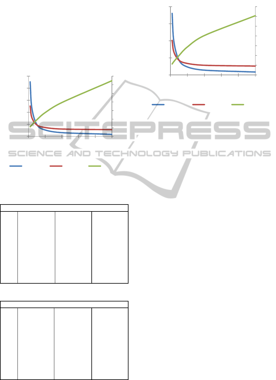
Additionally the ETs and quotients of the MINIP
results are shown exemplary in figure 3 (without
ERT) and in figure 4 (with ERT).
As explained in the introduction the multi-pass
raycasting consists of building the geometry first
before executing the raycasting itself. Due to the fact
that the geometry building remains almost constant
at about 0.5 to 0.6 milliseconds it is not included
separately in the tables and figures. (The multi-pass
execution times are the sum of all passes.)
Figure 3: ETs over step sizes (MINIP, without ERT) and
the quotient of multi-pass divided by single-pass times.
Table 2: Alpha Blending ET (times in milliseconds).
Alpha Blending
step
size
[mm]
single-pass multi-pass quotient
raycast ERT raycast ERT raycast ERT
0.001 275.2 147.3 117.2 76.3 0.4 0.5
0.002 146.2 81.9 73.6 52.2 0.5 0.6
0.005 63.0 38.0 44.7 37.1 0.7 1.0
0.01 33.8 21.0 35.0 31.8 1.0 1.5
0.02 18.3 12.5 28.7 28.5 1.6 2.3
0.05 9.8 8.4 26.8 26.4 2.7 3.1
Table 3: Gradient Calculation ET (times in milliseconds).
Gradient Calculation
step
size
[mm]
single-pass multi-pass quotient
raycast ERT raycast ERT raycast ERT
0.001 369.5 52.2 408.5 159.1 1.1 3.0
0.002 194.5 31.1 240.0 101.6 1.2 3.3
0.005 83.5 17.3 123.5 66.4 1.5 3.8
0.01 46.6 13.6 77.2 52.7 1.7 3.9
0.02 27.0 11.0 53.3 44.0 2.0 4.0
0.05 13.3 9.5 37.0 36.1 2.8 3.8
Figure 4: ETs over step sizes (MINIP, with ERT) and the
quotient of multi-pass divided by single-pass times.
4 DISCUSSION
The results show that the ERT can lower the ET up
to about 14% in the best case (Gradient Calculation,
single-pass, step size 0.001). At worst the ERT had
no influence on the ET (MINIP, single-pass, step
size 0.05). Hence the implementation of an ERT is
always advisable.
Furthermore the results show that the single-pass
implementation produces lower ETs than the multi-
pass one at step sizes larger than about 0.005 mm for
the MINIP (with and without ERT) and 0.01 mm for
the Alpha Blending (with and without ERT).
For the Gradient Calculation the results show that
the single-pass raycasting produces lower ETs for
the whole measurement. But the quotient reveals
that the multi-pass raycasting would produce lower
ETs for even smaller step sizes.
Smaller step sizes lead to higher computational
load for the fragment shader. As remarked in the
introduction the full computational load of the
fragment shader is the disadvantage of the single-
pass technique. When this load reaches a certain
value the performance lead changes from single-pass
technique to multi-pass technique.
Therefore, the reported comparison shows that
there is no general performance advantage for one of
the raycasting techniques. The ET of the respective
technique depends on the computational load of the
fragment shader and on the chosen raycasting type.
Further work is addressed to the determination of
the exact parameters that define which raycasting
technique should be preferred for which task.
Additionally the influence of more optimization
0,0
0,5
1,0
1,5
2,0
2,5
3,0
3,5
00
50
100
150
200
250
0 0,01 0,02 0,03 0,04 0,05
ET [ms]
step size [mm]
single-pass multi-pass quotient
0,0
0,5
1,0
1,5
2,0
2,5
3,0
3,5
00
50
100
150
200
0 0,01 0,02 0,03 0,04 0,05
ET [ms]
step size [mm]
single-pass multi-pass quotient
OpenGLSL-basedRaycasting-ComparisonofExecutionDurationsofMulti-passvs.Single-passTechnique
309

techniques (e.g. empty space skipping, culling
techniques) and the used graphics card will be
investigated.
ACKNOWLEDGEMENTS
This work was funded by the Landesregierung
Nordrhein-Westfalen in the Med in.NRW-program,
grant no. GW01-078.
REFERENCES
Kruger, J. and Westermann, R., 2003. Acceleration
Techniques for GPU-based Volume Rendering.
Proceedings of the 14th IEEE Visualization 2003
(VIS’03), p. 38.
Marques, R., Santos, L. P., Leskovsky, P. and Paloc, C.,
2009. GPU ray casting. Proceedings of the 17th
Encontro Portugeês de Computação Gráfica (EPCG
09), p. 83–91.
Matsui, M., Ino, F. and Hagihara, K., 2005. Parallel
Volume Rendering with Early Ray Termination for
Visualizing Large-Scale Datasets. Parallel and
Distributed Processing and Applications, pp. 245-256.
Mensmann, J., Ropinski, T. and Hinrichs, K., 2010. An
Advanced Volume Raycasting Technique using GPU
Stream Processing. GRAPP: International Conference
on Computer Graphics Theory and Applications, pp.
190-198.
Movania, M. M., 2013. OpenGL Development Cookbook.
Birmingham, UK: Packt Publishing.
Porter, T. and Duff, T., 1984. Compositing Digital Images.
SIGGRAPH Comput. Graph., July, pp. 253-259.
Radiopaedia.org, 2014. Radiopaedia. [Online] Available
at: http://radiopaedia.org/articles/minimum-intensity-
projection-minip [Accessed 11/16/2014].
Röttger, S. et al., 2003. Smart Hardware-Accelerated
Volume Rendering. Proceedings of EG/IEEE TCVG
Symposium on Visualization, pp. 231-238.
Shreiner, D., Sellers, G., Kessenich, J. and Licea-Kane, B.,
2013. In-Application Profiling. In: OpenGL
Programming Guide, Eighth Edition. Upper Saddle
River, NJ et al.: Addison-Wesley, pp. 881-883.
Vanecek, 2014. OpenGL4Net. [Online] Available at:
http://sourceforge.net/projects/ogl4net/ [Accessed
11/16/2014].
Venkataraman, S., 2009. 4D Volume Rendering. Silicon
Valley, s.n.
IVAPP2015-InternationalConferenceonInformationVisualizationTheoryandApplications
310
