Social-based Forwarding of Messages in Sensor Networks

Basim Mahmood, Marcello Tomasini and Ronaldo Menezes

BioComplex Laboratory, Department of Computer Science, Florida Institute of Technology, Melbourne, U.S.A.

Keywords:

Social Networks, Social Network of Sensors, Human Mobility.

Abstract:

As we adopt the Internet of Things (IoT), the boundaries between sensor and social networks are likely to

disappear. However, to this date, the use of social networks in the design of wireless sensor network protocols

has not received much attention. In this paper, we focus on the concept of information dissemination in a

framework where sensors are carried by people who are part of a social network. We propose two social-based

forwarding approaches for what has been called Social Network of Sensors (SNoS). To this end, we exploit

two important characteristics of ties in social networks, namely strong ties and weak ties. The former is used

to achieve rapid dissemination to nearby sensors while the latter aims at dissemination to faraway sensors.

1 INTRODUCTION

Wireless Sensor Networks (WSNs) are an important

area of research because they relate to many applica-

tions in the areas of transportation, military and agri-

culture. A typical WSN consists of many small de-

vices deployed over a geographical area, where each

device is called a Sensor and can measure environ-

mental or physical conditions (e.g., temperature) in

a particular area of interest. The structure of WSNs

can be static or dynamic. In a static WSN, sensors

are stationary while in a dynamic WSN, a sensor’s

position is subject to change. In this work, we de-

sign social-based approaches for message forwarding

in SNoS (Tomasini et al., 2013) inspired by the con-

cept of strong ties and weak ties. Following the def-

inition and the hypothesis of Granovetter (Granovet-

ter, 1973), we proposed information forwarding ap-

proaches to achieve nearby spreading of information,

called Strong-Ties-Based Forwarding (STBF), and

to achieve faraway spreading of information, called

Weak-Ties-Based Forwarding (WTBF).

2 RELATED WORKS

The idea behind data forwarding in WSNs is to mini-

mize the consumption of network resources by choos-

ing appropriate receivers (relays) in the forwarding

process (Lambrou and Panayiotou, 2009). In the net-

work literature, several forwarding approaches have

been described implementing different strategies.

Epidemic forwarding was proposed by Vahdat and

Becker (Vahdat et al., 2000). Data messages are sent

to all network nodes in the communication range of

a particular node, all nodes are guaranteed to receive

all data messages in the network. This approach has a

high level of ﬂooding due to the number of messages

exchanged which leads to waste network resources.

Yet, the Epidemic approach is widely used to bench-

mark other protocols.

PRoPHET was proposed by Lindgren et al. (Lind-

gren et al., 2003) and is based on a node’s history of

encounters, which means that if a node i encounters

another node j frequently, node i is more likely to en-

counter node j again in the future. With the encounter

ratios, a delivery predictability is calculated for each

node destination, the value of the delivery predictabil-

ity represents the chance to deliver a message to a par-

ticular destination.

Social ties in social networks have been studied by

Granovetter (Granovetter, 1973) who argued that so-

cial relations come in two kinds: strong and weak ties.

In social networks, these ties are used for different

purposes but weak ties are mostly important for indi-

viduals to receive information from faraway locations

in their network. These types can also be deﬁned in

the context of SNoS based on the sensor’s encounter

frequencies. That is, the strong ties of sensor i are the

other sensors whose encounter frequency to i is high.

By contrast, the weak ties are formed to those sensors

that have low encounter frequencies with sensor i.

Mahmood B., Tomasini M. and Menezes R..

Social-based Forwarding of Messages in Sensor Networks.

DOI: 10.5220/0005327700850090

In Proceedings of the 4th International Conference on Sensor Networks (SENSORNETS-2015), pages 85-90

ISBN: 978-989-758-086-4

 2015 SCITEPRESS (Science and Technology Publications, Lda.)

3 THE MODEL

We initially start with an environment that represents

a squared city of (6.2 × 6.2) sq. miles divided in

to squared blocks (100× 100 blocks). We deployed

2,040 mobile sensors in the environment, exponen-

tially distributed from the center of the city (envi-

ronment) since most metropolises follow this popula-

tion distribution (Grossman-Clarke et al., 2005). The

event that is used in the measuring of the informa-

tion dissemination is generated in a random location

which is then considered the center of the dissemina-

tion (for the purposes of measuring distances). The

communication between sensors is peer-to-peer. The

communication range of sensors (sensors’ radius) is

55 yards (50 meters) in line Wi-Fi communication

range. In the simulation environment, each sensor

moves at a ﬁxed speed of 1 block per tick (a tick is

equal to 1.2 minute in real time considering the nor-

mal human walking speed is ≈ 3.1 miles/h (≈ 5 km/h)

(Fitzpatrick et al., 2006). Sensors move according to

the Individual Mobility model proposed by Song et

al. (Song et al., 2010) because this model has the abil-

ity to accurately describe the characteristics of human

mobility. We provide the average of 100 runs for each

approach. The simulations stop when 90% of the net-

work knows about the event.

We proposed two novel forwarding approaches,

namely Strong-Ties-Based Forwarding (STBF) and

Weak-Ties-Based Forwarding (WTBF). These ap-

proaches are used for information dissemination,

where the spreading process is based on relation type

between sender and receiver(strong or weak relation).

Our proposal is that sensors can maintain the strength

of ties to use the strength to achieve different dissem-

ination patterns.

Each sensor in the simulation has to be able to

keep track of encounters with other sensors. For each

sensor, all encounters are memorized in a dynamic list

, where i represents a particular sensor in the en-

vironment. The items in this list represent the IDs

(e.g. MAC addresses) of the encountered sensors.

Each sensor has another dynamic list which is derived

from the T

list: the CST

list (the list of cumulative

strong ties) contains the sensors (candidates sensors)

that have strong ties with sensor i while the CWT

list

(the list of cumulativeweak ties) contains this list con-

tains the sensors (candidates sensors) that have weak

ties with sensor i. These derived lists are used respec-

tively by the STBF and WTBF approaches.

In STBF, we extract the strong ties for each sen-

sor from the T

list. As mentioned, the strong ties

emerge with people we associate with frequently and

frequency does not correlate with friendship. This

means, the strength of a tie represents frequency and

not afﬁnity between two individuals. The friendship

relation between two individuals may be derived from

the strength of the relation, but the distribution of

these encounters and their regularity also play a role

(Bulut and Szymanski, 2010; Vaz de Melo et al.,

2013; Bai and Helmy, 2004). For the purposes of

this work, friendship deﬁnition is not important, but

rather frequency; most of us meet many people fre-

quently without considering them as friends (e.g., at

work). The strong ties of a sensor can be extracted

by taking the higher frequency sensors in its history

of encounters (T

list). This process can be performed

based on the so-called “80/20” rule (Newman, 2005).

This rule states that for many observations, approxi-

mately 80% of the effects caused by the other 20%.

This rule is common in economical and natural pro-

cesses, for example, 80% of a company’s sales come

from 20% of its clients. Statistically, this rule is ap-

plicable to the applications that follow a power law

distribution (Newman, 2005). Based on this statistical

phenomenon(since the degree distribution of nodes in

our model follows a power law distribution), for each

sensor i we take the higher 20% frequencies items of

the T

list at time t, and inserting the corresponding

sensor ID into the CST

in which contains the ID’s of

the sensors that have the higher frequencies (strong

ties) of the T

list.

In WTBF, we insert the sensor ID of the lower

80% frequencies items of the T

list into the CWT

list

(weak ties). This process is performed by each sen-

sor at every time step of the simulation. In order to

have values that are statistically signiﬁcant, we em-

ploy (i) atraining procedure where we let all sensors

freely move in the environment in the absence of any

event for 100 time steps—this procedure represents a

proactive step before executing any of the approaches

we used in this work aiming to create a history of en-

counters and initiating the T

list for each sensor; then

we execute a (ii) checking procedure, at every time

step t and for each sensor i, the decision of insert-

ing an items into the CST

and CWT

lists is based on

Algorithm 1 which describes whether an element is

included in the CST

or in the CWT

of a particular

sensor. In our algorithm, we take into considerations

that a weak tie may, in the future, become a strong

tie. In this case, we remove this item from CWT

and

insert it into the CST

Once sensors have their CST

and CWT

lists (can-

didates lists), they can be used in the forwarding pro-

cess of STBF and WTBF respectively. This means a

sensor forwards data only to other sensors that are in

their candidates list. Furthermore, to carry out the for-

warding process, three conditions must be validated:

SENSORNETS2015-4thInternationalConferenceonSensorNetworks

Algorithm 1: Algorithm for inserting a sensor ID into the

CST

and CWT

. Note that t represents time.

for all ID ∈ higher 20% frequencies in T

(t) do

if ID 6∈ CST

then

add ID to CST

end if

if ID ∈ CWT

then

remove ID from CWT

end if

end for

for all ID ∈ lower 80% frequencies in the T

(t) do

if ID 6∈ CWT

then

add ID to CWT

end if

end for

• The receiver must not have the event.

• The forwarder and the receiver must be in the

communication range of each other.

• The receiver must be in the candidates list of the

forwarder.

The two approaches described (STBF and WTBF)

are designed to work in two modes:

Full Mode. In this mode, a sensor, i, forwards data

to all sensors in its candidates list (CST

and CWT

lists in STBF and WTBF respectively).

Partial Mode. A sensor has a predeﬁned number of

sensor(s) to forward data to (we used 1 to 5 re-

ceivers). These receivers must be selected from

sensor’s candidates list (CST

and CWT

4 EXPERIMENTAL RESULTS

We benchmark the proposed approaches by highlight-

ing their behavior according to two criteria: data-

spreading distance and data-spreading coverage area.

Moreover, for a deeper evaluation, we considered dif-

ferent scenarios for the Epidemic and PRoPHET ap-

proaches. In Epidemic forwarding, we forced it to

work in multiple mode in addition to its default work-

ing mode (all). In the default mode a sensor spreads

data randomly to all other sensors in its communica-

tion range, while in the multiple mode, we involve 1

to 5 receivers instead of considering all sensors as re-

ceivers. In PRoPHET, we involved 2 to 5 receivers

rather than 1 (the default working mode).

4.1 Spreading Distance

The control of the spread distance is the main contri-

bution of our approaches. We have proposed the two

approaches aiming at having some control of the dis-

tance the event generated in a sensor will travel. The

hypothesis that we adapted from social networks is

that strong ties will restrict the forwarding to nearby

sensors while the use of weak ties will spread the

information to the farthest distances; spread to far

distances may be useful to certain applications (e.g.,

emergency warnings).

The ﬁndings show that the farthest possible dis-

tance from the center of the simulation environment

can be obtained using the default mode of Epidemic

(up to 2.85 miles), followed by the full mode of

WTBF (up to 2.67 miles), and then by the full mode

of STBF (up to 2.26 miles), and ﬁnally, the default

mode of PRoPHET (up to 2.05 miles). This means

that WTBF can disseminate information to locations

as far as the ones done by a full Epidemic model.

For a detailed view to their behavior, we tested the

partial mode of STBF and WTBF, and the multiple-

message mode of the benchmarking approaches un-

der different number of receivers. It should be clar-

iﬁed that in Epidemic, when spreading to 1 sensor,

this sensor may have a strong tie to the forwarder be-

cause Epidemic discards the type of ties during the

spreading process. Therefore, this case may limit the

forwarding process to include only the surrounded

area (e.g., same group or community). Whereas in

WTBF, when spreading to 1 receiver, the receiver

will deﬁnitely have a weak tie to the forwarder. For

this reason, the partial mode version of WTBF with

1 receiver outperforms Epidemic and the other ap-

proaches as shown in Figure 1; this is a very inter-

esting result because it demonstrates that if we want

to maintain a low message overhead, WTBF can be a

better alternative for message dissemination to far lo-

cations than even Epidemic. Moreover, being able to

replicate such behavior in the context of mobile sen-

sor networks (or SNoS) conﬁrms the idea that a weak

tie plays a signiﬁcant role in data ﬂowing to different

social communities by acting as a bridge or a broker

(Granovetter, 1973).

Figure 1: Overall behavior in terms of spreading distance

when varying the number of receivers in each approach.

Furthermore, the results also show that the partial

mode of STBF underperforms the multiple mode of

Epidemic, and outperforms PRoPHET. Yet, the goal

Social-basedForwardingofMessagesinSensorNetworks

of STBF is to restrict the dissemination to nearby lo-

cations so the “underperforming” is actually the de-

sired outcome for STBF. In more details, Figure 1 ex-

hibits the average spreading distance that can be ob-

tained for each approach using different number of

receivers. We noticed that each approach reaches the

equilibrium when the number of receivers approxi-

mates 4 sensors, this can be interpreted as an indicator

of the convergence between both modes of the pro-

posed approaches at this level of receivers. However,

this exact level may vary depending on sensor density

within the simulation environment. In Figure 2 we

show the range of the distances that can be reached

for each approach. This ﬁgure also shows the lowest

and highest distances, the lower and upper quartiles,

and the median for each approach.

WTBF STBF PRoPHET Epidemic

1.6 2.0 2.4 2.8

Distance (miles)

Figure 2: The average distances for the full modes and par-

tial modes (using 1, 2, 3, 4, and 5 receivers) of the proposed

approaches and the single and multiple message modes of

the benchmarking approaches (using 1 to 5 receivers).

Figure 2 also allows us to observe that the varia-

tions achieved in WTBF and STBF are smaller than

the competition. WTBF can be said to be more re-

liable with the range of distance the event will reach

than Epidemic because the variance is smaller. Con-

versely, although PRoPHET can limit the spread to

very short distances, the variance is quite high when

compared to STBF.

4.2 Coverage Area

Data forwarding approaches try to cover as much area

as possible in the network environment. The efﬁ-

ciency of these approaches in terms of coverage area

depends on the size of the area they cover which

in general should be maximized, and the consump-

tion of network resources which should be minimized

(Gaudette et al., 2014). Recall that our simulation en-

vironment is 38.61 sq. miles (or a square of 6.2× 6.2

miles). In this evaluation, we calculate the minimum

and the maximum areas that can be covered by the

event during the spreading process, these areas can be

deﬁned as follows:

Minimum Coverage Area: part of the area that is

always under the coverage of data spreading.

Maximum Coverage Area: part of the area which is

not always under the coverage of data spreading

but has been reached at least once.

As mentioned, we have 100 runs for each ap-

proach in our experiments, each run gives a particular

coverage area. The intersection region of these ar-

eas represents the minimum coverage area, while the

union of all the runs represents the maximum cover-

age area. We can clearly see that the disparity in the

areas between the minimum and the maximum is very

small (Figure 3). Table 1, illustrates the obtained re-

sults and their proportion to the environment area for

each approach. We observe the following points:

• Minimum and maximum areas that can be cov-

ered using WTBF and Epidemic are very close.

• WTBF outperforms PRoPHET and STBF. This is

expected since we want STBF to dissimulate the

event around the location where it appeared.

• The intensity of data spreading is very high in Epi-

demic and very low in WTBF.

• STBF covers more area than PRoPHET in both

the maximum and the minimum coverage area.

However, STBF has higher intensity in data

spreading than PRoPHET.

Given that STBF is proposed to avoid the spread-

ing of information to faraway places, we had to inves-

tigate a little more what was taking place as the result

above seems to negate our hypothesis of strong ties

being useful for information dissemination to nearby

locations. However, results in Figure 3 can be a side-

effect of the settings of our model which stops when

90% of the network knows about the event.

Hence, we changed the stop condition to be in-

dependent of the number of sensors knowing about

the event. We provide two other tests (each of 100

runs) with different stop conditions. First, running

the simulator for 100 time ticks (Test 2) and then for

50 time ticks (Test 3). Figures 4 and 5 show mini-

mum and maximum coverage area for each approach.

We can observe that the disparity between the mini-

mum and the maximum areas is more prominent than

what we see in Figure 3. These new results reﬂect

better the behavior of both WTBF and STBF conﬁrm-

ing the hypothesis that weak ties spread events farther

than strong ties. Tables 2 and 3 show the results of

100 ticks and 50 ticks respectively, and their propor-

tion to the environment area. Lastly, we measured the

proportion of the minimum to the maximum cover-

age area of each approach for every test. Clearly, the

proportions for 100 ticks and 50 ticks resemble Gra-

novetter’s work better than the experiment using 90%

of the sensors as shown in Table 4.

SENSORNETS2015-4thInternationalConferenceonSensorNetworks

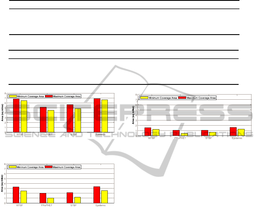
Table 1: Minimum and maximum coverage areas with the experiment runs until 90% of the sensors know about the event.

Epidemic PRoPHET STBF WTBF

Maximum Coverage Area Area (sq. mile) 6.87 5.09 5.62 6.80

the proportion to the total area 17.80% 13.20% 14.55% 17.60%

Minimum Coverage Area Area (sq. mile) 6.62 4.49 4.82 6.43

the proportion to the total area 17.15% 11.64% 12.50% 16.65%

Table 2: Minimum and maximum coverage area when the simulation runs for 100 ticks.

Epidemic PRoPHET STBF WTBF

Maximum Coverage Area Area (sq. mile) 3.36 2.01 2.13 3.27

the proportion to the total area 8.72% 5.20% 5.51% 8.47%

Minimum Coverage Area Area (sq. mile) 2.55 1.04 1.21 2.48

the proportion to the total area 6.60% 2.70% 3.13% 6.42%

Figure 3: Minimum and the maximum coverage area when

using the simulator with a condition to stop based on 90%

of the sensors knowing about the event.

Figure 4: minimum and maximum coverage area when us-

ing the settings of the experiment in which the sensors are

allowed to work for 100 ticks of the simulation.

5 CONCLUSIONS AND FUTURE

WORKS

We analyzed the proposed protocols based on two

criteria: data-spreading distance and data-spreading

coverage area. Furthermore, we measured the inten-

sity of message-spreading in the environment and de-

livery time for all the approaches in this work. We

can summarize STBF and WTBF approaches by giv-

ing some recommendations when designing a SNoS:

• If the goal is to forward data to the farthest dis-

tance, the best option is to use the partial mode

of WTBF, because its results reﬂect a good per-

formance in terms of distance and the number of

messages exchanged. However, we should not ig-

Figure 5: minimum and maximum coverage area when us-

ing the settings of the experiment in which the sensors are

allowed to work for 50 ticks of the simulation.

nore the fact that WTBF approach spends more

time than the other approaches.

• If we are looking to forward data to a wider cover-

age area with low data spreading intensity we can

choose WTBF.

• If the goal is reducing the number of messages

exchanged within the network, we recommend

WTBF approach.

In this work, we did not investigate the issue

spreading direction. However, as the future work, we

are planning to investigate this issue using our pro-

posed approaches. It is important to ﬁnd whether the

social network reconstructed from IM models lead to

a bias towards certain directions in the environment.

Finally, the environment we currently use does not

assume the existence of barriers or obstacles which

may be common in urban environments. It may be

interesting to investigate how the proposed forward-

ing mechanisms perform under conﬁgurations with

obstacles (representing, for instance, buildings in a

city). We believe the results will not change because

the mobility model used has been shown to approxi-

mate human mobility in urban areas. In fact, the data

used to evaluate the IM model comes from real cellu-

lar data in large cities.

Social-basedForwardingofMessagesinSensorNetworks

Table 3: Minimum and maximum coverage area when the simulation runs for only 50 ticks.

Epidemic PRoPHET STBF WTBF

Maximum Coverage Area Area (sq. mile) 1.62 1.05 1.06 1.56

the proportion to the total area 4.21% 2.73% 2.74% 4.04%

Minimum Coverage Area Area (sq. mile) 1.30 0.47 0.68 1.22

the proportion to the total area 3.37% 1.22% 1.76% 3.15%

Table 4: proportion of the minimum to the maximum coverage area for all the approaches using all three experiments.

Epidemic PRoPHET STBF WTBF

90% of the sensors reached 96.3% 88.2% 85.7% 94.5%

Simulation runs for 100 ticks 75.8% 51.7% 56.8% 75.8%

Simulation runs for 50 ticks 80.2% 44.7% 64.1% 78.2%

REFERENCES

Bai, F. and Helmy, A. (2004). A survey of mobility mod-

els. Wireless Adhoc Networks. University of Southern

California, USA, 206.

Bulut, E. and Szymanski, B. K. (2010). Friendship based

routing in delay tolerant mobile social networks.

In Global Telecommunications Conference (GLOBE-

COM 2010), 2010 IEEE, pages 1–5. IEEE.

Fitzpatrick, K., Brewer, M. A., and Turner, S. (2006). An-

other look at pedestrian walking speed. Transporta-

tion Research Record: Journal of the Transportation

Research Board, 1982(1):21–29.

Gaudette, B., Hanumaiah, V., Krunz, M., and Vrudhula, S.

(2014). Maximizing quality of coverage under con-

nectivity constraints in solar-powered active wireless

sensor networks. ACM Trans. Sen. Netw., 10(4):59:1–

59:27.

Granovetter, M. S. (1973). The strength of weak ties. Amer-

ican journal of sociology, pages 1360–1380.

Grossman-Clarke, S., Zehnder, J. A., Stefanov, W. L., Liu,

Y., and Zoldak, M. A. (2005). Urban modiﬁcations in

a mesoscale meteorological model and the effects on

near-surface variables in an arid metropolitan region.

Journal of Applied Meteorology, 44(9):1281–1297.

Lambrou, T. P. and Panayiotou, C. G. (2009). A survey on

routing techniques supporting mobility in sensor net-

works. In Mobile Ad-hoc and Sensor Networks, 2009.

MSN’09. 5th International Conference on, pages 78–

85. IEEE.

Lindgren, A., Doria, A., and Schel´en, O. (2003). Proba-

bilistic routing in intermittently connected networks.

ACM SIGMOBILE Mobile Computing and Communi-

cations Review, 7(3):19–20.

Newman, M. E. (2005). Power laws, pareto distributions

and zipf’s law. Contemporary physics, 46(5):323–

351.

Song, C., Koren, T., Wang, P., and Barab´asi, A.-L. (2010).

Modelling the scaling properties of human mobility.

Nature Physics, 6(10):818–823.

Tomasini, M., Zambonelli, F., and Menezes, R. (2013). Us-

ing patterns of social dynamics in the design of social

networks of sensors. In 2013 IEEE and Internet of

Things (iThings/CPSCom), pages 685–692. IEEE.

Vahdat, A., Becker, D., et al. (2000). Epidemic routing for

partially connected ad hoc networks. Technical report,

Technical Report CS-200006, Duke University.

Vaz de Melo, P. O., Viana, A. C., Fiore, M., Jaffr`es-Runser,

K., Le Mou¨el, F., and Loureiro, A. A. (2013). Recast:

Telling apart social and random relationships in dy-

namic networks. In Proceedings of the 16th ACM in-

ternational conference on Modeling, analysis & simu-

lation of wireless and mobile systems, pages 327–334.

ACM.

SENSORNETS2015-4thInternationalConferenceonSensorNetworks