Arc and Swarm-based Representations of Customer’s Flows among

Supermarkets

Evgheni Polisciuc

, Pedro Cruz

, Hugo Amaro

, Catarina Maçãs

, Tiago Carvalho

, Frederico Santos

and Penousal Machado

CISUC, Department of Informatics Engineering, University of Coimbra, Coimbra, Portugal

Sonae, Maia, Portugal

Keywords:

OD Visualization, Flow Visualization, Geo-temporal Visualization, Big Data.

Abstract:

Representing large amounts of ﬂows involves dealing with the representation of directionality and the re-

duction of visual cluttering. This article describes the application of two ﬂow representation techniques to

the visualization of transitions of customers among supermarkets over time. The ﬁrst approach relies in arc

representations together with a combination of methods to represent directionality of transitions. The other

approach uses a swarm-based system in order to reduce visual clutter, bundling edges in an organic fashion

and improving clarity.

1 INTRODUCTION

Nowadays data are collected faster than analyzed.

The advances in computation allow the storage and

processing of large amounts of data in a reasonable

time. Additionally, current visualization techniques

enable efﬁcient analysis of data, while trying to deal

with generated visual clutter in order to achieve better

visual clarity. Graphical exploratory analysis of tran-

sitions in space is important to many ﬁelds of study,

since it enables the understanding of the amounts of

ﬂows among geographical locations, while enabling

to focus on certain geographical areas and time spans.

In this article we present an application of visual

techniques to represent big amounts of consumption

data in more than 700 supermarkets and hypermar-

kets in Portugal, having all registered transactions

from May of 2012 to April of 2014. This article

focuses on the graphical exploration of customers’

transitions among supermarkets over time. Transi-

tions are visualized in order to reveal ﬂow patterns

of customers. We considered a transition whenever

there is a change in a transaction’s location in a cus-

tomer’s shopping history. These transitions can be

represented as origin-destination (OD) vectors. The

reasons that cause a transaction can be fairly intricate,

but can perhaps be related with local and temporal

discounts, and seasonal and deﬁnite changes in a cus-

tomer’s residency.

This paper tackles the visualization of ﬂows of

transitions using two approaches. More precisely,

the issue of visual clutter in high-dense representa-

tion and the directionality of ﬂow streams. The ﬁrst

approach employs a well known visualization tech-

nique, which is based on arc representation (sec-

tion 3 provides a detailed description of the applica-

tion of this technique to our data). The second ap-

proach relies on bio-inspired mechanism known as

ﬂocking. The application of this technique enables

the representation to convey information on transition

ﬂows with bio-inspired aesthetics while reducing the

amount of visual clutter to improve clarity (see sec-

tion 4 for a detailed description).

2 BACKGROUND AND RELATED

WORK

Arc diagrams are a widely known method to visual-

ize structures in text, songs or any other sequences of

symbols popularized by Wattenberg M. (Wattenberg,

2002). Since then, arcs have been applied in differ-

ent domains, namely in graph visualization and geo-

graphic visualization, particularly to represent origin-

destination data. The work of Schich et al. (Schich

et al., 2014) is an example of application of arcs in

geographic context to represent OD-like data. In this

300

Polisciuc E., Cruz P., Amaro H., Maçãs C., Carvalho T., Santos F. and Machado P..

Arc and Swarm-based Representations of Customer’s Flows among Supermarkets.

DOI: 10.5220/0005316503000306

In Proceedings of the 6th International Conference on Information Visualization Theory and Applications (IVAPP-2015), pages 300-306

ISBN: 978-989-758-088-8

 2015 SCITEPRESS (Science and Technology Publications, Lda.)

work origin and destination represents, respectively,

the place of birth and place of death of notable people

in the history. The directionality is represented with

color interpolation (red-blue for origin-destination).

One of the concerns of origin-destination visualiza-

tion is the representation of directionality of edges,

particularly when dealing with bidirectional ﬂows.

Recent work (Holten and van Wijk, 2009) has pre-

sented six different ways of edge directionality repre-

sentation (tapered, dark-to-light, light-to-dark, arrow,

curved, and green-to-red) and compared the reading

performance of each technique. This study suggests

that the tapered method is advantageous in most situa-

tions, unlike curved representation which is the worst

of all cases. In any cases, the representation of bidi-

rectional data is still challenging, due to additional vi-

sual information added to each edge.

Direct visualization of large volumes of OD data

generates high degrees of visual clutter. In these

cases a reduction strategy known as edge bundling

can be applied, which is characterized not only by

graph simpliﬁcation, but also by the revelation of

principal streams of ﬂow. Holten introduced edge

bundling for compound graphs. His work consisted of

routing edges through a hierarchical layout using B-

Splines (Holten, 2006). There are several variations

of edge bundling starting with force-directed (Holten

and Van Wijk, 2009) up to sophisticated kernel den-

sity estimation strategies (Hurter et al., 2012). Gener-

ally, edge bundling consists of drawing similar edges

on the same path, i.e. edges that are related in geom-

etry and direction are routed along the same path.

In the geographic context OD representation as a

rule refers to the ﬂow visualization (also known as

ﬂow maps), which is deeply rooted in the history of

information visualization. Early examples, such as

wine exports from France, produced by Minard (Tufte

and Graves-Morris, 1983, page: 25), represents quan-

tity as well as direction of wine exports encoded by

the thickness of the corresponding edges, which dis-

join from the parent edge. The work of Phan et al.

(Phan et al., 2005) describes an automated approach

to the generation of ﬂow maps using a hierarchical

clustering algorithm, given a series of nodes and ﬂow

data. Generally, in geographic context ﬂow visual-

ization refers to the representation of amounts of any

type of variables that move from one location to an-

other (e.g. migrations, transportation of goods, etc.).

The advantage of ﬂow maps is that they reduce visual

clutter by merging edges. However, they present a

series of of problems, such as the perception of direc-

tionality of ﬂow, when large amounts of bidirectional

OD data is considered.

3 DATA DESCRIPTION

Our dataset consists of 278GB of information about

customer purchases in 729 supermarkets and hyper-

markets in Portugal in a time span of 24 months

(from May, 2012 until April, 2014), including the

geo localization of 682 supermarkets, as well as the

regions of the country they belong to. The dataset

comprises approximately 2.86 billions of transactions

where each transaction has the following attributes:

customer card id, amount spent, product designation,

quantity of the purchased products and the date and

time of the transaction. It is important to note that

several individuals may hold the same customer card

with an unique client id (e.g. members of a family).

The dataset has a total of 6.6 Million unique card ids.

Before the extraction of transitions among super-

markets we ﬁrst compute their geographical clusters.

The reason for that is because the majority of super-

markets belong to shopping centers which are consid-

ered as a unique geographical location. In this case

the DBSCAN algorithm (Ester et al., 1996) was ap-

plied with the parameters of 0 for K and 0.01 for ep-

silon. As a result 304 clusters were obtained, where

the extracted locations are the centroids of the clusters

of supermarkets (each centroid will be referenced as

a single supermarket for the sake of simplicity).

With the clusters computed we proceed to ex-

tract transitions as follows: ﬁrst the data is aggre-

gated by day (24 hours); then for each client the

sequence of transitions is computed by excluding

subsequences of repeated places. For example, let

X = (A,A,B,B,B,C) be the sequence of supermarkets

where a client made transactions. So, the transition

sequence would be X

= (t

(A,B),t

(B,C)).

4 ARC REPRESENTATION

Our ﬁrst approach was based on direct representation

of the data. The transition sequence is directly en-

coded by edges, that represents the link between the

origin-destination supermarket, as well as the num-

ber of clients that transitioned. The directionality of

the edge is represented based on the combination of

taped and curved methods, due to the bidirectionally

of data. Since arc-based approach usually do not rep-

resent directionality, the thickness of arcs in our visu-

alization increase as they approach their destination,

resembling the trajectory of a projectile or a comet.

The asymmetrical curve gives a more natural sense

of direction. Arcs where also used because they re-

duce visual clutter when compared with straight lines

methods.

ArcandSwarm-basedRepresentationsofCustomer'sFlowsamongSupermarkets

301

4.1 Arc Anatomy

The arcs consist of a bezier curve (Farin et al., 2002,

page: 4-6) with two control points (see Figure 1).

These points are the vertices of triangles ODC1 and

DOC2. The two triangles are computed differently

with empirically determined values. The length of

the DC1 edge has 60% of the length of OD, and the

angle β is equal to 27

. The OC2 edge has 90% of

the length of OD, and the angle α varies proportion-

ally to the OD length, and is constrained to the range

[10

, 20

]. The upper and lower angular limits cor-

respond to the maximum and minimum length of the

set of ODs. By adjusting the C2 control point the arc

changes its curvature, making the long arcs visually

distinct from short ones.

Figure 1: The position of control points for different OD

distances.

The arc on its own does not convey any informa-

tion besides the connection of two points. In order

to encode the quantity of clients involved in the same

transitions we use the thickness and transparency of

the line (Figure 2). The thickness give a good estima-

tion of the encoded value, while opacity diminishes

the impact of less relevant transitions. Only the des-

tination side of the arc changes its thickness, interpo-

lating from the destination value (amount of transi-

tioned clients) to a certain minimum at the opposite

side of the arc. Moreover, this kind of representa-

tion gives a clear understanding of the direction of OD

data (Holten and van Wijk, 2009).

The color of each arc varies with respect to the

corresponding value. The minimum and maximum

numbers of transitions are represented with blue and

orange respectively, and intermediate colors are inter-

polated according to the value (Figure 2). Therefore,

arcs that represent few transitions appear in transpar-

ent blue color, unlike arcs that represent high number

of transitions, which appear in saturated orange color.

4.2 Application

Each day in the dataset is visualized separately dis-

playing only the transitions that occurred on that par-

Figure 2: Arcs representing the data variable. Reading top

down each arc represents maximum, 75% quartile, median

and 25% quartile value. The colors are interpolated in the

range RGBA[(86,150,255,30),(255, 152, 74,100)].

ticular day. By navigating on the timeline the user

can change the current day. Although, we can zoom

to any part of the country to analyze it in detail, we

focused on two major metropolitan areas -– Porto and

Lisbon — and in a general view of the country (Figure

3). In the general view all the arcs whose origin and

destination locations are inside the same region are

not represented, since the density of such transitions

at this zoom level does enable a proper representation

beyond visual noise. Therefore, in the general view

we opted to visualize only inter-regional transitions.

In closer views we only display the arcs that ﬁt in the

viewing area.

While applying this technique to the dataset we

noted several limitations. First, a large data density

generates a high degree of visual clutter, making gen-

eral view hard to analyze (Figure 3, image on the left).

For instance edges that connect supermarkets in Lis-

bon and supermarkets in Porto hide a signiﬁcant part

of the edges that connect other urban areas, for ex-

ample Coimbra and Porto. Also, in our data the most

of the transitions occur within shorter distances limit-

ing this approach in terms of analysis, since it is ex-

tremely difﬁcult to estimate the values and direction

of short arcs (See for example Figure 3, images in the

middle and on the right).

5 SECOND APPROACH

In the second approach we relied on nature-inspired

mechanisms, more precisely on a swarm system.

Each transition in the sequence is encoded through

a simulated path of a boid. By running the system

each boid interacts with the ghosts of other boids

(Reynolds, 1987), updating its own path at each sim-

IVAPP2015-InternationalConferenceonInformationVisualizationTheoryandApplications

302

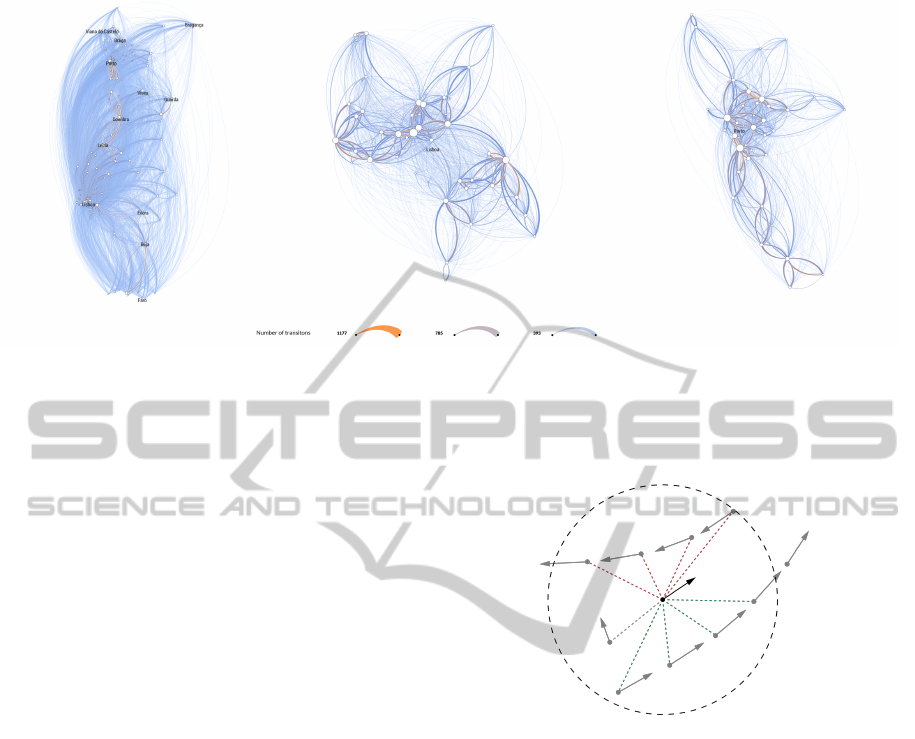
Figure 3: The general view of Portugal (left), metropolitan area of Porto (middle), metropolitan area of Lisbon (right). The

displayed date is 23 of December, 2012. The scale of the zoomed views with respect to the general view is 1:10.

ulation step. Ghosts of each boid hold information

about the position, direction, destination and data

value at each simulation point on the path. The pro-

cess is iterative and in each execution cycle all the

active boids are simulated.

5.1 Flocking and Flow Representation

In order to reﬂect the ﬂowing nature of the informa-

tion we resort to a swarm system, which is comprised

by artiﬁcial agents (boids) that react to the presence

and characteristics of neighboring boids. While run-

ning the system each boid simulates the ﬂow of data,

adapting the paths that represent OD edges, bundling

them and making visual patterns emerge. As a result,

the visualization represents the ﬂows in the dataset

with reduced degree of visual clutter.

Each boid in the system is characterized by di-

rection, speed, radius of vision, the number of tran-

sitions that it represents, a set of behavioral rules, and

its unique origin-destination points. During the simu-

lation each boid leaves persistent traces, further refer-

enced as ghosts, that contain information for the speed

and position at that point as well as a reference to the

boid itself.

The behavioral rules of each boid are determined

through the interaction with the traces of other mem-

bers of the ﬂock. Pairwise comparison between boids

and ghosts establishes the relationship between them

and their behavior. If the agents advance in similar di-

rections, they are considered “friendly”. If the agents

advance in opposite directions, they are considered

“unfriendly”. Otherwise, they ignore each other. The

degree of similarity affects the force of attraction

or repulsion between agents and ghosts. Therefore,

friendly agents advance together as a group and un-

friendly agents repel from each other avoiding colli-

sions. Figure 4 illustrates this behavior.

Figure 4: Pairwise comparison between one boid and neigh-

boring ghosts. The black dot and the arrow in the center are

the current boid and its direction. The gray dots are ghosts

left by other boids. The dashed circle is the radius of vi-

sion and the dashed lines are the relations with the ghosts –

green and red lines represent friendly and unfriendly rela-

tionships, respectively. Gray dashed line connects the ghost

that is ignored.

The direction and the speed of each boid B with

position ~p

depends on the position ~p

of ghosts X

within the radius of vision d

V R

and the angle between

their direction vectors

and

. Each boid in the

system simulates its path until reaching its destina-

tion. Otherwise, the boid ﬁnishes its simulation and

is marked as inactive. The following rules are applied

to each active boid in the system.

Stick with friends. Each boid attempts to move

towards the center of the group of friendly ghosts.

Friendly ghosts are determined by the angle between

directions of the boid and neighbor ghosts. Their

similarity creates stronger relationship and are deter-

mined by the distance and the angle between their di-

rections.

ArcandSwarm-basedRepresentationsofCustomer'sFlowsamongSupermarkets

303

| ~p

− ~p

| ≤ d

V R

[

< a

max

)

⇒ ~v

∑

− ~p

| ~p

− ~p

w(X, B) (1)

Avoid unfriendly boids. Each boid attempts to

avoid collision with the ghosts of other boids if the an-

gle between their directions are bigger than π − a

max

| ~p

− ~p

| ≤ d

V R

[

< π − a

max

)

⇒ ~v

∑



− ⊥

w(X,B) i fC

( ~p

) ≥ 0

⊥

w(X,B) i fC

( ~p

) < 0

(2)

Similarity between two boids determines the

weight of the force, and is related to the distance be-

tween boids, the angle between their directions, and

the data value, this is, the quantity of transactions that

are encoded. Boids that contain higher quantities have

greater impact over the other members of the ﬂock.

So, the similarity between two boids is computed as

follows:

w(X,B) =

(

) + w

( ~p

, ~p

)

× data

(3)

(

) = 1 −





[

max





(4)

( ~p

, ~p

) = 2

(2−0.1

| ~p

− ~p

(5)

Where d

and d

are the vectors of the direction

of boid B and ghost X, and a

max

is the maximum an-

gle allowed between two direction vectors. dataX

is the normalized value of data variable ((value −

min)/(max − min)). All the parameters were empiri-

cally determined.

Avoid static points. Every boid B in the system at-

tempts to avoid collision with the static points S with

the position ~c

, which is the centroid of a cluster of

supermarkets. The origin and destination points do

not enter in the calculation.

|~c

− ~p

| ≤ d

⇒ ~v

∑



− ⊥

i f C

(

) ≥ 0

⊥

i f C

(

) < 0

(6)

(~p) =



~p − ~p



(7)

Finally, each boid is always attracted by its desti-

nation, having the force vector equal to the normal-

ized vector pointing towards the boid’s destination.

When the boid approximates its destination, all the

forces, except the destination force, are ignored and

the speed is limited to 1. This restriction ensures that

each boid reaches its destination.

The location of boids is deﬁned by applying the

computed vector forces as follows: all the forces are

added to the acceleration; then the acceleration is

added to the speed; ﬁnally, the speed is limited to the

predeﬁned maximum and is added to the current lo-

cation. The maximum deﬁned speed reﬂects on the

visual output resulting in high and low curvature of

edges for speed limited to 1 and 3, respectively.

In each iteration the boid’s paths are updated ac-

cording to the current state of the system. More pre-

cisely, during the execution cycle each boid interacts

with the ghosts left by other boids and never with their

own ghosts. The process stops when the boid reaches

its destination or its path remain unaltered during last

three simulation steps. In order to determine if a path

has changed since the last iteration we compute the

root-mean-square deviation (RMSD) at each iteration.

So, given the current path P

and the previous path P

which comprise sequences of ghosts P computed in

current and the last iteration, RMSD is calculated as

follows:

RMSD =

∑

− P

(8)

Where n is the minimum number of ghosts in both

paths. If the average of the last three RMSD is below

a certain threshold (in our case 0.5) then the boid is

marked as inactive preventing it from further updating

of its path.

The application of this technique to the data has

similar aspects with the ﬁrst approach -– focus on the

general view and two zoomed views for Lisbon and

Porto metropolitan areas. In the general view all the

supermarkets that belong to the same region are not

considered, while in the zoomed views the edges that

do not ﬁt in the zoomed area are not computed. The

number of transitions per path is encoded by the thick-

ness of the line and by the color scheme used in arc

representation. The directionality is represented using

the tapered method (see Fig. 5).

At this stage we found limitations in our approach.

First there is no guaranty that the algorithm con-

verges, since it highly depends of the overall state of

the system, which varies according to the data. For

that reason we established a threshold equal to 99.9%

of inactive boids to force the algorithm to stop. The

complexity of the algorithm also depends on data,

more precisely it depends on the number of OD edges

and their length, since each boid computes its position

by considering the trails of every other boid and more

lengthy edges implies that more trails are generated.

6 DISCUSSION

In this section, arc representation, swarm-based rep-

resentation and force directed edge bundling (FDEB)

IVAPP2015-InternationalConferenceonInformationVisualizationTheoryandApplications

304

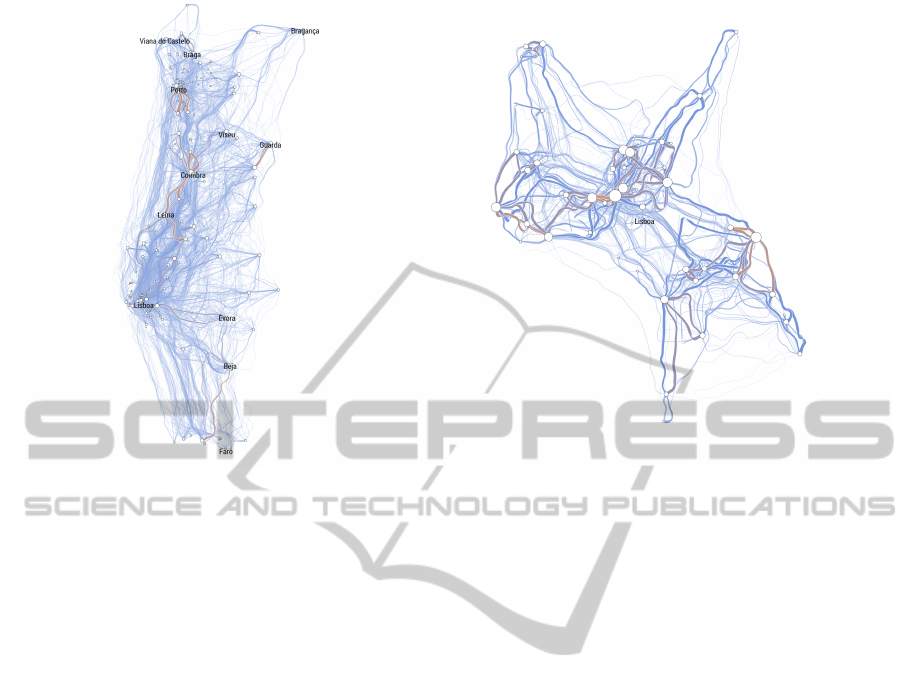
Figure 5: General view of Portugal, image on the left, and metropolitan area of Lisbon, image on the right. The displayed

date is 23 of December, 2012.

are compared and discussed. The visual output from

the three techniques is displayed in Figure 6. To com-

pare the approaches we choose a day before Christ-

mas (23 of December of 2012) and zoomed on Lis-

bon’s view. The same visual mapping is applied in

all three approaches allowing a fair comparison be-

tween them. The usage of the color and the thickness

of edges was described in previous sections.

The very ﬁrst comparison reveals the efﬁciency

of visual clutter reduction. As can be observed, the

force directed edge bundling method generates less

visual clutter in comparison with arc and swarm-

based representation. Also, swarm-based visualiza-

tion is less cluttered than arc representation. When

using swarms, main streams of ﬂow are visually dis-

tinct from each other leaving enough space for the

ones with less impact.

In the swarm system each boid attempts to avoid

the boids with opposite directions, as such the simu-

lated paths are never routed through the same trail,

making it possible to distinguish paths that encode

opposite directions. As can be observed, this isn’t

the case when using the FDEB, and the arc methods.

These algorithms do not take into account the direc-

tionality of streams, which is an emergent character-

istic of the swarm-based approach. Finally, since the

boids in the system attempt to avoid static points, the

Supermarkets, nodes encoded with white circles, are

clearly visible and do not visually interfere with the

lines drawn by the swarming algorithm.

7 CONCLUSIONS AND FUTURE

WORK

In this article we have presented two graphical ex-

plorations of transitions among supermarkets. In the

ﬁrst approach we explored direct representation of

transition sequences. This consists of the combina-

tion of curved and taped strategies to represent origin-

destination data, which enables the perception of bidi-

rectional edges. The shape of the arcs, inspired on the

trajectory of launched projectiles, enforces the read-

ability of direction. The number of clients, whose

transition is represented by an arc, is encoded by the

line thickness, and by color.

The second approach overcomes the cluttering is-

sue in the visualization compared to the ﬁrst one. This

approach consists of a set of boids that represent each

transition with their paths. Each singe boid follows

simple behavioral rules by pairwise interaction with

other neighbor boids. When two neighboring boids

advance in the similar direction they are considered

as friends and attempt to move together. In contrast,

when two neighboring boids have opposite directions

they are considered as not friends and attempt to avoid

each other. Otherwise, they ignore each other. The

relation between two boids is determined by the dis-

tance between them and the angle between their direc-

tions. The boids that represent more customers have

higher impact on other members of the system. Fi-

ArcandSwarm-basedRepresentationsofCustomer'sFlowsamongSupermarkets

305

Figure 6: Three approaches for representing OD data. Force directed edge bundling (left), arc-based representation (middle)

and swarm-based representation (right). Displayed metropolitan area of Lisbon on 23 of December of 2012.

nally, every boid attempts to avoid static points, ex-

cept when these are located nearby the origin or the

destination point.

The arcs visualization for large volumes of origin-

destination data generates high degree of visual clut-

ter. In contrast, our swarm-based approach simpliﬁed

the visualization representing the ﬂow data in a nat-

ural and organic manner, but is computationally in-

tensive when high volumes of data are considered.

The force directed edge bungling method generates

even less visual clutter in comparison with our ap-

proaches. However, the swarm-based representation

visually separates the streams of ﬂow with opposite

directionality, which does not happens in force di-

rected edge bundling.

As future work we will improve the performance

of our swarm-based approach, for example by using

a quadtree structure to store and gain faster access

to nearby ghost boids. In order to further improve

the efﬁciency of the technique, the algorithm can up-

date existing ghost boids with new information in-

stead of indeﬁnitely adding new ghost boids to the

same quadtree cell.

ACKNOWLEDGEMENTS

This research is partially funded by: iCIS project

(CENTRO-07-ST24-FEDER-002003), which is co-

ﬁnanced by QREN, in the scope of the Mais Centro

Program and European Union’s FEDER; Sonae Viz

— Big Data Visualization for retail.

REFERENCES

Ester, M., Kriegel, H.-P., Sander, J., and Xu, X. (1996).

A density-based algorithm for discovering clusters in

large spatial databases with noise. In Kdd, volume 96,

pages 226–231.

Farin, G. E., Hoschek, J., and Kim, M.-S. (2002). Handbook

of computer aided geometric design. Elsevier.

Holten, D. (2006). Hierarchical edge bundles: Visualization

of adjacency relations in hierarchical data. Visualiza-

tion and Computer Graphics, IEEE Transactions on,

12(5):741–748.

Holten, D. and Van Wijk, J. J. (2009). Force-directed edge

bundling for graph visualization. In Computer Graph-

ics Forum, volume 28, pages 983–990. Wiley Online

Library.

Holten, D. and van Wijk, J. J. (2009). A user study on visu-

alizing directed edges in graphs. In Proceedings of the

SIGCHI Conference on Human Factors in Computing

Systems, pages 2299–2308. ACM.

Hurter, C., Ersoy, O., and Telea, A. (2012). Graph bundling

by kernel density estimation. In Computer Graphics

Forum, volume 31, pages 865–874. Wiley Online Li-

brary.

Phan, D., Xiao, L., Yeh, R., and Hanrahan, P. (2005). Flow

map layout. In Information Visualization, 2005. IN-

FOVIS 2005. IEEE Symposium on, pages 219–224.

IEEE.

Reynolds, C. W. (1987). Flocks, herds and schools: A dis-

tributed behavioral model. ACM SIGGRAPH Com-

puter Graphics, 21(4):25–34.

Schich, M., Song, C., Ahn, Y.-Y., Mirsky, A., Mar-

tino, M., Barabási, A.-L., and Helbing, D. (2014).

A network framework of cultural history. science,

345(6196):558–562.

Tufte, E. R. and Graves-Morris, P. (1983). The visual dis-

play of quantitative information, volume 2. Graphics

press Cheshire, CT.

Wattenberg, M. (2002). Arc diagrams: Visualizing structure

in strings. In Information Visualization, 2002. INFO-

VIS 2002. IEEE Symposium on, pages 110–116. IEEE.

IVAPP2015-InternationalConferenceonInformationVisualizationTheoryandApplications

306