Bio-inspired Model for Motion Estimation using an Address-event
Representation
Luma Issa Abdul-Kreem
1,2
and Heiko Neumann
1
1
Inst. for Neural Information Processing, Ulm University, Ulm, Germany
2
Control and Systems Engineering Dept., University of Technology, Baghdad, Iraq
Keywords:
Event-based Vision, Optic Flow, Neuromorphic Sensor, Neural Model.
Abstract:
In this paper, we propose a new bio-inspired approach for motion estimation using a Dynamic Vision Sensor
(DVS) (Lichtsteiner et al., 2008), where an event-based-temporal window accumulation is introduced. This
format accumulates the activity of the pixels over a short time, i.e. several µs. The optic flow is estimated by a
new neural model mechanism which is inspired by the motion pathway of the visual system and is consistent
with the vision sensor functionality, where new temporal filters are proposed. Since the DVS already gener-
ates temporal derivatives of the input signal, we thus suggest a smoothing temporal filter instead of biphasic
temporal filters that introduced by (Adelson and Bergen, 1985). Our model extracts motion information via a
spatiotemporal energy mechanism which is oriented in the space-time domain and tuned in spatial frequency.
To achieve balanced activities of individual cells against the neighborhood activities, a normalization process
is carried out. We tested our model using different kinds of stimuli that were moved via translatory and rotatory
motions. The results highlight an accurate flow estimation compared with synthetic ground truth. In order to
show the robustness of our model, we examined the model by probing it with synthetically generated ground
truth stimuli and realistic complex motions, e.g. biological motions and a bouncing ball, with satisfactory
results.
1 INTRODUCTION
High temporal resolution, low latency and large dy-
namic range visual sensing are key features of the
address-event-representation (AER) principle, where
each pixel of the vision sensor responds indepen-
dently and almost instantaneously translates local
contrast changes of the scene into events (ON or
OFF). This principle is used in our study to profit from
the advantage of the event-based technology instead
of using standard frame-based camera technology. A
frame-based imager transmits moving scenes into a
series of consecutive frames. These frames are con-
structed at a fixed time rate, which generates an enor-
mous amount of redundant information. In contrast,
a Dynamic Vision Sensor (DVS) reduces this redun-
dancy using a new technology inspired by visual sys-
tems. The functionality of this sensor is similar to the
biological retina, where a stream of spike events are
generated as a polarity format ON (+1) or OFF (-1)
if a positive or negative contrast change is detected.
No changes in contrast, on the other hand, produce
zero output, and as a consequence, any such redun-
dant information sampled by frame-based cameras is
reduced.
A DVS has high temporal resolution, where the
events are generated asynchronously and sent out al-
most instantaneously on the address bus. Thus, subtle
and fast motions can be detected. In addition, a DVS
has low latency and a large dynamic range due to the
pixels locally responding to relative changes in inten-
sity. A DVS’s ability to produce an event at 1 µs time
precision and a latency of 15µs with bright illumina-
tion were illustrated in (Lichtsteiner et al., 2008).
The new sensor technology has led to several re-
cent applications in many fields to exploit the advan-
tages of DVSs compared with traditional frame-based
imagers, where several application-oriented studies
have capitalized on those features. Such works in-
clude (Litzenberger et al., 2006a) and (Delbruck
and Lichtsteiner, 2008), where Litzenberger and co-
authors introduced an algorithm that used the silicon
retina imager to estimate vehicle speed based on the
slope of the events cloud. Delbruck and co-authors
presented a hybrid neuromorphic procedural system
for object tracking via an event driven cluster tracker
335
Abdul-Kreem L. and Neumann H..
Bio-inspired Model for Motion Estimation using an Address-event Representation.
DOI: 10.5220/0005311503350346
In Proceedings of the 10th International Conference on Computer Vision Theory and Applications (VISAPP-2015), pages 335-346
ISBN: 978-989-758-091-8
Copyright
c
 2015 SCITEPRESS (Science and Technology Publications, Lda.)

e
1
(p)
e
2
(p)
e
n
(p)
t
e
on
(p) + e
o
( p)
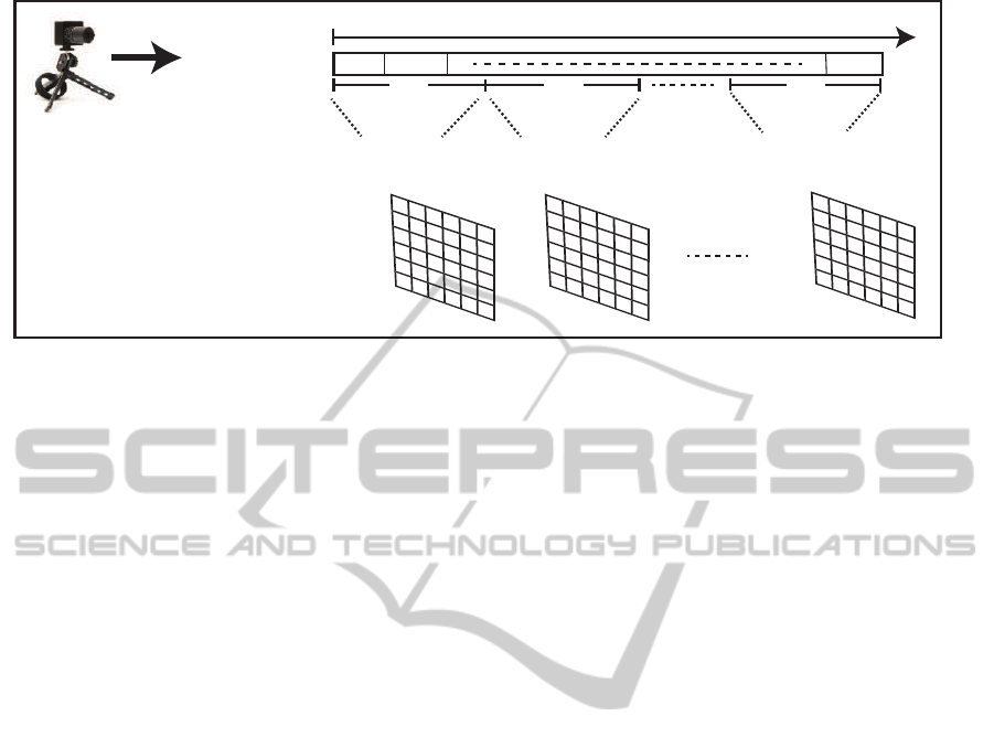
Events stream
Event-based-temporal window
e
on
(p) + e
o
(p)
e
on
(p) + e
o
(p)
∑
t=0
∆t
1
∑
t=0
∆t
1
∑
t=∆t
1
∆t
2
∑
t=∆t
1
∆t
2
∑
t=∆t
n-1
∆t
n
∑
t=∆t
n-1
∆t
n
∆t
1
∆t
2
∆t
n
Figure 1: Event-based-temporal window accumulation. An event stream is represented as a sequence of events e at a position
p and time t. e
on
and e
of f
identify the event activity (+1) ON and (-1) OFF, respectively.
algorithm. The authors showed how a moving ball
can be detected, tracked and successfully blocked by
a goalie robot despite a low contrast object and com-
plex background. The event-cluster algorithm was in-
troduced by (Litzenberger et al., 2006b) and (Ni et al.,
2011), where a first study considered a real world ap-
plication, namely vehicle tracking for traffic monitor-
ing in real time, and a second study addressed micro-
robotics tracking.
Motion estimation is an advanced topic in auto-
mated visual processing and has been investigated
widely using conventional cameras (see, e.g., (Horn
and Schunck, 1981), (Brox et al., 2004) and (Drulea
and Nedevschi, 2013)). Few studies have been pub-
lished using the new vision sensor technology of
an address-event silicon retina. Benosman and co-
authors (Benosman et al., 2012) implemented the en-
ergy minimization method introduced in (Lucas and
Kanade, 1981) to calculate motion flow using an
event-based retina. Since the vision sensor generates
a stream of events (ON or OFF) and does not pro-
vide gray levels, the authors suggested using pixel ac-
tivities by integrating events within a short temporal
window. Gradients were estimated by comparing ac-
tive pixels over one temporal window to calculate the
spatial gradient, and two temporal windows to calcu-
late the temporal gradient. A least squares error mini-
mization technique was used to calculate the local op-
tic flow based on such pixel neighborhoods. Benos-
man and co-authors showed beneficial results, how-
ever, their methods to approximate local gradients of
the luminance function from event-sequences has its
limitations and in some cases leads to inconclusive re-
sults (see (Tschechne et al., 2014a)).
Recently (Tschechne et al., 2014b) presented an
algorithm for motion estimation where the authors
utilized spatiotemporal filters of the type suggested
by findings of (De Valois et al., 2000) to estimate a
local motion flow calculated for each event occurring
in the scene. The spatiotemporal filters were imple-
mented over a spatial buffer of (11×11) which stores
the timestamp of the events. This method is character-
ized as a neuroscience approach and showed adequate
results, however, the aperture problem needs to be ad-
dressed.
The motion estimation field using address event
representation thus requires further investigation and
development. In this paper, we introduce a bio-
inspired model following the energy model of (Adel-
son and Bergen, 1985), where a new set of tempo-
ral filters are proposed which are compatible with the
vision sensor functionality. Since one event is not
suitable for spatiotemporal energy models, an event-
based-temporal window is suggested as a time sam-
pling technique to accumulate the events over a short
temporal interval. Our model shows accurate mo-
tion estimations with a small error margin compared
against synthetic ground truth. The following section
details our methodology and the subsequent sections
outline the results along with a comparison against
(Tschechne et al., 2014b).
2 METHODOLOGY
2.1 Initial Input Representation from
ON/OFF Events
Our approach uses the event-based-temporal window
as a temporal sampling technique, where pixel activ-
ity , ON (+1) and OFF (-1), is accumulated separately
as below:
VISAPP2015-InternationalConferenceonComputerVisionTheoryandApplications
336

E(p,m) =
∆t
m
∑
t=∆t
m−1
e
on
(p,t) +
∆t
m
∑
t=∆t
m−1
e
of f
(p,t), m = [1,n], (1)
∆t
m
represents a variable interval length of the
sampling temporal window; e
on
(p,t) and e
of f
(p,t)
are ON and OFF events respectively, which occurred
at position p = (x,y) and time t. The main differ-
ences between an event-based-temporal window ac-
cumulation and a conventional frame-based imager
are: we integrate the events using a weighted tempo-
ral window of shorter duration, i.e. several µs, while
conventional frame-based integration is over approx-
imately 41.7 ms to achieve 24 frames/sec. In addi-
tion, the window can be locked at an event that oc-
curs. This introduces more flexibility since the stan-
dard frame-based acquisition is fixed and externally
synchronized. Thus, this sequence of the event-based-
temporal window will be exploited for motion esti-
mation. The event-based-temporal window accumu-
lation can be described as in Figure 1.
2.2 Detection of Motion Energy from
Event Input
Motion estimation using spatiotemporal filters emu-
lates motion detection processing of the primary vi-
sual cortex (Adelson and Bergen, 1985), where the
space-time filters are 3D and can here be decomposed
into separable products of two 2D spatial and two 1D
temporal kernels. The two spatial filters consist of dif-
ferent phases (evenand odd) while the temporal filters
consist of two different temporal integration windows
(fast and slow). The spatial receptive fields (RFs) of
odd and even filters can be implemented using Ga-
bor functions, which provide a close description of
the receptive fields in primary visual cortex area (V1)
(Ringach, 2002). We thus used these functions to
build even and odd spatial filters as in Eqs.(2) and (3),
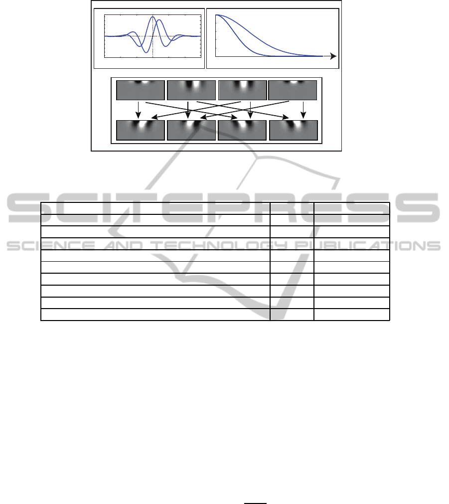
respectively, and shown in Figure 2 (a), namely
F
even
(p,θ
k
, f
s
) =
1
2πσ
2
s
· exp(−
˘x
2
+ ˘y
2
2σ
2
s
) ·cos(2π f
s
˘x),
(2)
F
odd
(p,θ
k
, f
s
) =
1
2πσ
2
s
· exp(−
˘x
2
+ ˘y
2
2σ
2
s
) ·sin(2π f
s
˘x),
(3)
where

ˇx
ˇy

=

cosθ
k
−sinθ
k
sinθ
k
cosθ
k

·

x
y

, θ
k
is the
spatial filter orientation with N different orientations
where k = {1,2,3...N} , σ
s
is the standard deviation
of the spatial filters and f
s
represents the spatial fre-
quency tuning.
In the model of (Adelson and Bergen, 1985) the
authors suggested to utilize temporal gamma func-
tions of different duration in order to accomplish tem-
poral smoothing and differentiation, leading to a tem-
porally biphasic response shape. In order to transcribe
this functionality to the AER output of the sensor, we
make use of the following approximation: The bipha-
sic Adelson-Bergen temporal filters can be decom-
posed into a convolution of numerical difference ker-
nel (to approximate a first-order derivative operation)
with a temporal smoothing filter. The event-based
sensor already operates to generate discrete events
based on changes in the input and, thus, generates
temporal derivatives of the input signal. For that rea-
son, we employ plain temporal smoothing filters and
convolve them with the input stream of events to ob-
tain scaled versions of temporally smoothed deriva-
tives of the input luminance function. Figure 2 (b)
shows the proposed temporal filters with two differ-
ent temporal integration windows (fast and slow). The
temporal filters can be written as
T
fast
(t) = exp(−
t
2
2σ
2
fast
) ·H(t), (4)
T
slow
(t) = exp(−
t
2
2σ
2
slow
) ·H(t), (5)
where σ
fast
, σ
slow
represent standard deviation of
the fast and slow temporal filters and H(t) denotes the
Heaviside step function (Oldham et al., 2010), which
generates the one-sidedness of temporal filters.
The opponent energy of the spatiotemporal filters
is calculated according to the scheme proposed in
(Adelson and Bergen, 1985), where the spatiotempo-
ral separable responses are obtained through the prod-
ucts of two spatial and two temporal filters responses
as shown in the first row of Figure 2 (c). These re-
sponses are combined in a linear fashion to get the
oriented selectivity responses as shown in the second
row of Figure 2 (c). The oriented linear combinations
are denoted by
F
v1
a
(x,y,θ
k
, f
s
,t) = F
even
(x,y,θ
k
, f
s
) ·T
slow
(t) +
F
odd
(x,y,θ
k
, f
s
) ·T
fast
(t), (6)
F
v1
b
(x,y,θ
k
, f
s
,t) = F
even
(x,y,θ
k
, f
s
) ·T
fast
(t) −
F
odd
(x,y,θ
k
, f
s
) ·T
slow
(t), (7)
F
v1
c
(x,y,θ
k
, f
s
,t) = F
even
(x,y,θ
k
, f
s
) ·T
slow
(t) −
F
odd
(x,y,θ
k
, f
s
) ·T
fast
(t), (8)
F
v1
d
(x,y,θ
k
, f
s
,t) = F
even
(x,y,θ
k
, f
s
) ·T
fast
(t) +
F
odd
(x,y,θ
k
, f
s
) ·T
slow
(t). (9)
Bio-inspiredModelforMotionEstimationusinganAddress-eventRepresentation
337

t
0
1
Temporal lters
a
b
c
Spatial lters
! " # 0 # "
!
$
%&'
%&!
%&"
%&#
0
%&#
%&"
%&!
%&'
1
+++ +- +- +
Figure 2: Spatiotemporal filter construction. (a) Spatial filters. (b) Temporal filters. (c) The first row represents the products
of two spatial and two temporal filters; the second row represents the sum and difference of the product filters.
Table 1: Parameters used in our model.
Definition variable value
Spatial filter frequency f
s
0.27
Sampling temporal window ∆t
m
25msec
Motion directions θ 0
◦
,45
◦
,90
◦
,135
◦
Standard deviation of spatial filters σ
s
1.5 pixel
Number of motion directions N 4
Standard deviation of slow temporal filter σ
slow
2.5 pixel
Standard deviation of fast temporal filter σ
fast
1 pixel
Standard deviation of Gaussian function normalization σ 4 pixel
leakage activities A 0.001
The opponent energy response for an event-based-
temporal window input E(p,n
t
) can be achieved
through nonlinear combinations of contrast invariant
responses (local spatial coordinate and feature selec-
tivities are omitted for better readability):
r
v1
= 4(([F
v1
a
∗ E]
2
+ [F
v1
b
∗ E]
2
) −
([F
v1
c
∗ E]
2
+ [F
v1
d
∗ E]
2
)), (10)
where ∗ indicates convolution. Since we used N
orientations (indicated by the 2D spatial filters) with
two directions (left vs. right relative to the orienta-
tion axis), the positive and negative responses of r
v1
indicate that the direction of motion is θ
k
and −θ
k
re-
spectively, hence 2N directions can be estimated.
2.3 Response Normalization
The activity in neurons show significant nonlinearities
depending on spatio-temporal activity distribution in
the cell activation in the space-feature domain sur-
rounding a target cell (Carandini and Heeger, 2012).
Such response nonlinearities have been demonstrated
in the LGN, early visual cortex (area V1), and be-
yond. In theoretical studies (e.g. (Brosch and Neu-
mann, 2014)) it has been proposed that such compres-
sion of stimulus responses can be achieved through
the normalization of the target cell response defined
by the weighted integration of activities in a neigh-
borhood defined over the space-feature domain of a
target cell. In other words the normalization operation
utilizes contextual information from a local neighbor-
hood that is defined in space as well as feature do-
mains relevant for the current computation. Such a
normalization can be generated at the neuronal level
by divisive, or shunting, inhibition (Dayan and Ab-
bot, 2001) and (Silver, 2010). Given the activity of
a neuron (defined by its membrane potential) the rate
of change can be characterized by the following rate
equation (Grossberg, 1988)
τ
dv(t)
dt
= −A· v(t) + (B−C· v(t)) · net
ex
−
(D+ E · v(t))· net
in
, (11)
given A representing the passive leakage, B and D are
parameters to denote the saturation potentials (relative
to C and E, respectively), and net
ex
and net
in
denote
generic excitatory and inhibitory inputs to the target
cell.
In order to achieve balanced cell activations
against the pool of neighboring cells, a normaliza-
tion is generated, following(Bouecke et al., 2010) and
VISAPP2015-InternationalConferenceonComputerVisionTheoryandApplications
338

(Brosch and Neumann, 2014). We employ a spatial
weighting function Λ
pool
σ
which realizes a distance-
dependent weighting characteristics, e.g., Gaussian.
The size of this neighborhood function is larger than
the receptive field, or kernel, size of the cells under
consideration. After normalization of activations, the
responses are guaranteed to be bounded within a lo-
cal activity range. In addition, a spectral whitening
of the local response distribution occurs (Lyu and Si-
moncelli, 2009).
We realized a slightly simplified version of the
scheme described in (Brosch and Neumann, 2014)
and solve the normalization interaction at equilib-
rium, namely evaluating the state response for
dv(t)
dt
=
0. Ever further, we set C = D = 0 in eq.(11) to define
a pure shunting inhibition, and B = E = 1 to scale the
response levels accordingly. As a consequence, we
get the steady state response for eq.(11) which reads
v
∞
=
net
ex
A+ net
in
. (12)
We normalize the motion energy r
v1
in the spatial
domain using an integration field that weights the ac-
tivities in the spatial neighborhood of the target. We
propose a spatial weight fall-off in accordance to a
Gaussian weighting function. The motion selective
responses are defined in direction space relative to the
local contrast orientation θ of the spatial filter kernels
used. We take the direction feature space into account
as well by calculating the average activity over all di-
rections. In all, we can denote the overall pool activa-
tion by
r
pool
(i, j) =
1
2N
∑
θ

r
v1
θ
∗ Λ
σ

ij
, (13)
with θ denoting the orientation selectivities,
′
∗
′
denotes the (spatial) convolution operator, (i, j) rep-
resents the spatial position of the cell, N is the num-
ber of contrast filter orientations and Λ is the weight-
ing function of the spatial pooling operation. The lat-
ter is parametrized by the parameter σ to denote the
width of the spatial extent. The resulting normalized
response is finally calculated by
r
nor
(i, j) =
r
v1
(i, j)
A+ r
pool
(i, j)
, (14)
A denotes a small constant that prevents from zero
division.
3 EXPERIMENTAL SETUP AND
RESULTS
3.1 Ground Truth Data
To evaluate our method, a set of different stimuli with
translatory and rotational motions were recorded us-
ing the DVS128 sensor. The rotational and transla-
tory motions were generated using linear and rota-
tional actuators, in which the linear actuator’s speed is
1.7 cm/sec and the rotational actuator’s speed is 2.62
rad/sec. The DVS sensor was mounted on a tripod
and placed 25 cm away from the stimulus.
The model parameters used for the illustrated re-
sults are shown in Table 1. The estimated results of
the optic flow were based on the maximum response
of r
V1
which generates a confidence for the mo-
tion direction (u
e
(p) v
e
(p))
T
= max
θ
r
v1
(p,θ, f
s
,t) ·
(cosθ − sinθ)
T
. Figures 3 and 4 present the transla-
tory and rotational motion results respectively, where
the stimulus image, a snippet of the event-based-
temporal window and ground truth are presented in
the first column. The second column shows the esti-
mated flow of the stimulus. In order to measure the
accuracy of our approach, we calculated the angular
error Φ(p) = cos
−1
(V
e
(p)·V
g
(p))/(|V
e
(p)||V
g
(p)|),
where V
e
(p)
T
= (u
e
(p),v
e
(p)) and V
g
(p)
T
=
(u
g
(p),v
g
(p)) represent the estimated and ground
truth flow vectors at position p, respectively. The er-
ror value in the range of [0
◦
,180
◦
] are depicted as a
histogram is shown in the third column.
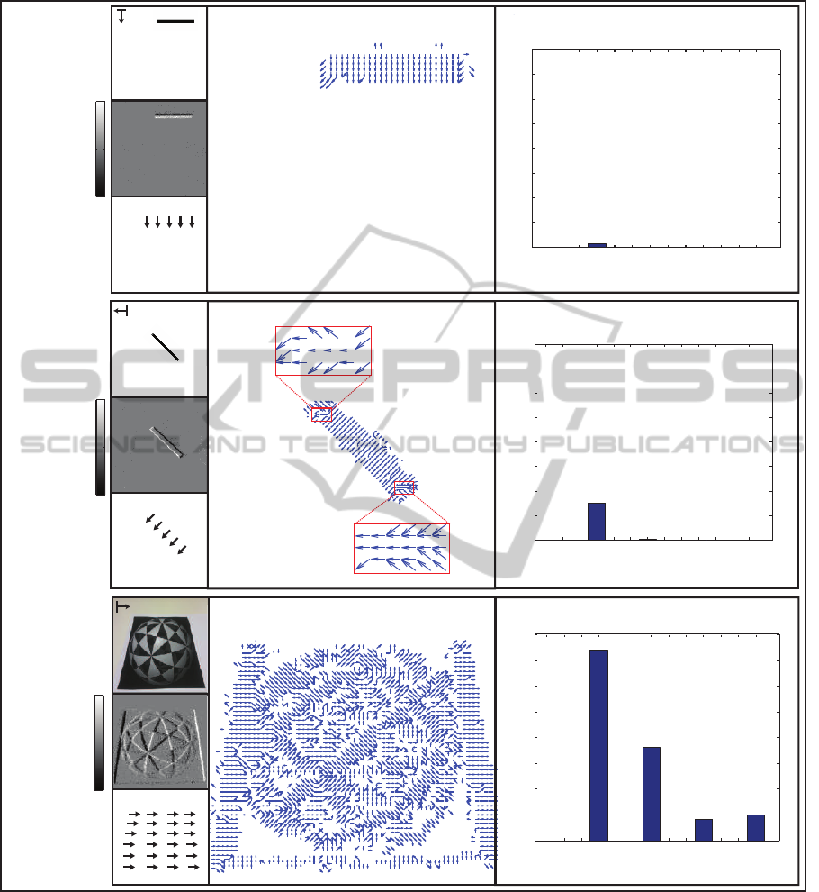
In case of translatory motion, we used three stim-
uli: a straight bar, a slanted bar (45
◦
) and a com-
plex picture in which different directions were se-
lected to movethese stimuli. The straight bar stimulus
was moved vertically down the field of view, while
the slanted bar and complex picture were moved to
the left and right, respectively. For the straight bar,
the angular error between the estimated flow and the
ground truth flow reveals that most of our event-
based-temporal window motions were estimated with
correct directions. In the slanted bar, however, the
angular error demonstrated the majority of the flow
in 45
◦
which referred to the motion was estimated as
orthogonal to the contrast (aperture problem, see sec-
tion 3.3). This is because the motion was estimated in
a local surround in which the size of the 2D spatial fil-
ter kernels is 9 × 9 pixels while the size of the slanted
bar is 11× 38 pixels, nevertheless a proper motion es-
timation was achieved at the bar ends. The aperture
problem can be resolved via the feedback of larger in-
tegration receptivefield MT cells (for more details see
(Bayerl and Neumann, 2004)). In the complex pic-
Bio-inspiredModelforMotionEstimationusinganAddress-eventRepresentation
339

!
0 !
OFF
ON
Straight-bar
! 0 !
OFF
ON
Complex-picture
! 0 !
OFF
ON
Slanted-bar
0
!""
1000
#!""
2000
$!""
3000
%!""
4000
#!
o
30
o
&!
o
60
o
'!
o
90
o
#"!
o
120
o
(#%!
o
#!"
o
(#)!
o
180
o
#!
o
30
o
&!
o
60
o
'!
o
90
o
#"!
o
120
o
(#%!
o
#!"
o
(#)!
o
180
o
0
!""
1000
#!""
2000
$!""
3000
%!""
4000
#!
o
30
o
&!
o
60
o
'!
o
90
o
#"!
o
120
o
(#%!
o
#!"
o
(#)!
o
180
o
0
!""
1000
#!""
2000
$!""
3000
%!""
4000
Figure 3: Processing results of translatory motion stimuli, straight-bar, slanted-bar and complex-picture. The first column of
each stimulus contains the input image, a snippet of the event-based-temporal window and sketch of the ground truth optical
flow field. The second column represents the estimated motion. The third column represents the histogram of the angular
error between the estimated motion and their respective ground truth, where the abscissa represents the binning in the rang of
the angular error Φ that are combined into one frequency bar [θ − 7.5
◦
,θ + 7.5
◦
), and the ordinate represents the number of
pixels.
ture, the angular error histogram showed some spu-
rios flow in 45
◦
due to the small slanted lines (aperture
problem). Moreover, a smaller spurious flow occured
in 90
◦
, 135
◦
and 180
◦
due to the low resolution of
DVS (128×128) which gives rise to spatial aliasing.
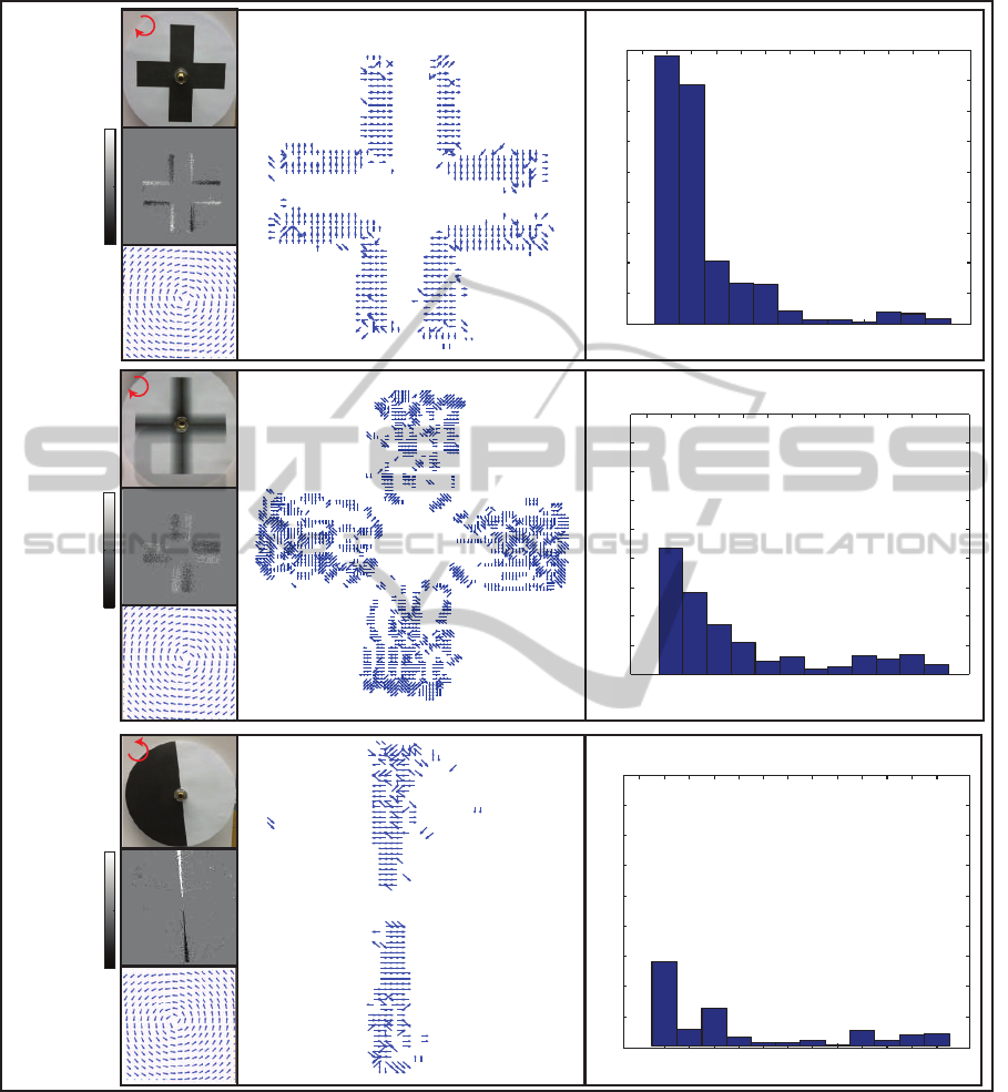
In the case of rotational motion, again three stim-
uli were used: black-cross, smooth-cross and half-
circle. These stimuli were rotated clockwise and
VISAPP2015-InternationalConferenceonComputerVisionTheoryandApplications
340

Black-cross
Half-circle
Smooth-cross
!
0 !
OFF
ON
!
0 !
OFF
ON
!
0 !
OFF
ON
0
100
200
300
400
!""
600
700
800
900
0
100
200
300
400
!""
600
700
800
900
0
100
200
300
400
!""
600
700
800
900
#!
o
30
o
$!
o
60
o
%!
o
90
o
#"!
o
120
o
&#'!
o
#!"
o
&#(!
o
180
o
#!
o
30
o
$!
o
60
o
%!
o
90
o
#"!
o
120
o
&#'!
o
#!"
o
&#(!
o
180
o
#!
o
30
o
$!
o
60
o
%!
o
90
o
#"!
o
120
o
&#'!
o
#!"
o
&#(!
o
180
o
Figure 4: Processing results of rotational motion stimuli, black-cross, smooth-cross and half-circle. The first column of each
stimulus contains the input image, a snippet of the event-based-temporal window and the ground truth optical flow field. The
second column represents the estimated motion. The third column represents the histogram of the angular error between
the estimated motion and their respective ground truth (error calculation considered the events positions), where the abscissa
represents the binning in the rang of the angular error Φ that are combined into one frequency bar [θ−7.5
◦
,θ+7.5
◦
), and the
ordinate represents the number of pixels.
counter clockwise, as highlighted in the top-left of the
stimulus images. In the black-cross stimulus, the mo-
tion estimation showed a flow pattern on the stimulus
edges, while the flow was lacking over the stimulus
interior due to the absence of contrast changes. We
repeated the test using a similar stimulus with gray-
level smoothing in the interior (smooth-cross stimu-
lus). Here the estimated result showed a flow motion
Bio-inspiredModelforMotionEstimationusinganAddress-eventRepresentation
341

over the interior as well as the edges of the stimulus.
In the half-circle stimulus, the stimulus was rotated
counter clockwise and the results showed a flow mo-
tion over the stimulus diagonal along the elongated
contrast edge contour. All rotated stimulus results re-
vealed appropriate flow estimation compared with the
ground truth of the clockwise and counter-clockwise
rotation in which most of the angular error was sand-
wiched between 15
◦
and 30
◦
.
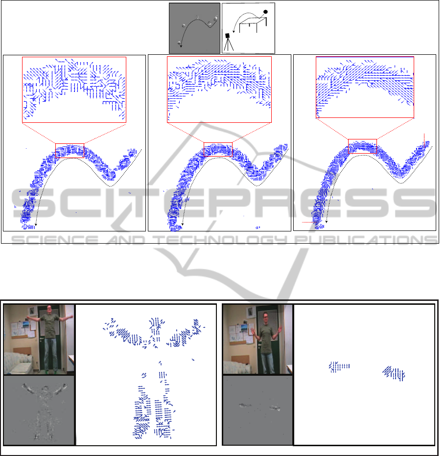
3.2 Complex Realistic Movements
To demonstrate the usefulness of our model under re-
alistic acquisition conditions, we extended our evalu-
ation to include bouncing ball and articulated biolog-
ical motion , Figures 5 and 6. In the case of bouncing
ball, different projected velocities occur since the ball
moves from a distant position towards the camera.
This leads to the additional challenge for our model
to estimate the motion when different velocities oc-
cur. We tested the influence of the temporal sampling
window size on the motion estimation using three dif-
ferent window sizes, 41.7msec, 15msec and 5msec, in
which the first temporal sampling is equivalent to the
typical sampling rate of a conventional frame-based
imager. Figure 5 shows that the motion estimation
can be improved with decreasing the temporal win-
dow size. This referred to the higher sampling rate
interval can capture small number of events and in-
stantaneously transcribe their motion in contrast to
the larger interval window that integrates more events
over time space which leads to lose the intermedi-
ate motion details. In general, the result of smaller
number of events acquisition, Figure 5 (c), shows a
proper estimation of flow direction comparing with
other sampling cases. In the same Figure, the ball
is approaching the DVS in which the speed of (B
2
)
is higher than (B
1
). The speed estimation should be
carried out at MT level, where the neurons are speed
selective (Perrone and Thiele, 2001). This extension
is currently under investigation and beyond the scope
of this article.
Our model was tested using biological motions in
which a real complex-articulated motion can be rep-
resented. Figure 6 shows two actions (jumping-jack
and two hands waving) of an actor, where different
movements and speeds were generated from body and
limbs motions. The estimated motions for the two ac-
tions have been done using sampling rate of 25 msec
in which a beneficial flow motions were obtained.
3.3 Comparison and Model Evaluation
We compared our results with those achieved in
(Tschechne et al., 2014b) using selective translatory
and rotationary motion stimuli, where the black-cross
and half-circle were used as rotational motion, and
straight stimulus was used as translatory motion. We
calculated the mean value of the angular error for
both approaches by comparing each estimated mo-
tion with their respective ground truth. The straight
bar stimulus revealed a mean value of 9.24
◦
com-
pared to 21.38
◦
in favor of the new approach. In the
black-crossand half-circle stimuli, the mean error val-
ues of our approach were 35.8
◦
and 34.8
◦
, while in
the (Tschechne et al., 2014b) they were 38.34
◦
and
41.8
◦
. The reason for the high error value in rotational
motion is that the rotational ground truth was built
based on continuous flow motion, while our model
estimates eight directions. Thus the error value can
be decreased by increasing the number of estimated
directions for each of the models investigated.
To evaluate the effect of the spatial filters fre-
quency f
s
, we calculated the motion using three dif-
ferent values of f
s
(0.27
◦
,0.3
◦
and 0.35
◦
) for a selec-
tive stimulus, half-circle. The results revealed mean
error values o f(32.53
◦
,43.9
◦
and 69.36
◦
). These re-
sults indicated that f
s
has an impact on the estimated
motion in which 0.27 gives the best result. In order
to show the robustness of our model with (Tschechne
et al., 2014b), we estimated the motion for both mod-
els using similar values σ
s
= 4, f
s
= 0.14 and kernel
size 15× 15 pixels. The results revealed a mean error
value of 8.44
◦
compared to 19.29
◦
in favor of the new
approach. In general, the calculated mean errors indi-
cate that our model could estimate the motion with a
smaller initial error detection than the model proposed
in (Tschechne et al., 2014b).
3.4 Aperture Problem and IOC
Mechanism
Neurons in the primary visual cortical area V1 that
are selective to spatio-temporal stimulus features have
small RFs, or filter sizes. Consequently, they can only
detect local motion components that occur within
their RFs. That means that along elongated contrasts
only ambiguous motion information can be detected
locally. It is the normal flow component that can be
measured along the local contrast gradient of the lu-
minance function (aperture problem). In our test sce-
narios this has been investigated with input shown in
Figure 3 (slanted bar). The aperture problem can be
resolved either by utilizing local feature responses at
corners, line ends, or junctions that belong to a single
surface to betracked. Another approachis to integrate
several normal flow estimates at distant locations. The
integration strategy might be either based on vector
VISAPP2015-InternationalConferenceonComputerVisionTheoryandApplications
342

DVS
B
1
B
2
b
c
a
Figure 5: Estimated motion of bouncing ball: The first row depicts the experimental setup and samples of ball events. The
second row shows the optic flow for the ball path. (a) sampling duration is 41.7msec. (b) sampling duration is 15msec. (c)
sampling duration is 5msec. The time period of (a), (b) and (c) is 0.64 sec. B
1
and B
2
represent two points located at different
position on the path of the ball motion in which the speed values are different
a
b
Figure 6: Estimated motion of articulated motion of an actor. (a) Jumping-jack. (b) Two hands waving. The small figures
represent an original image from the video and a snippet of an events-based-temporal window. The large figures represent the
estimated motions.
integration (VA) ((Yo and Wilson, 1992)) or on the
intersection-of-constraints (IOC) mechanism, as sug-
gested by (Adelson and Movshon, 1982). The latter
approach can be demonstrated to calculate the exact
movement of, e.g., two overlapping gratings which
move translatory behind a circular aperture in distinct
directions (plaid). If the two gratings have same con-
trast and spatial frequency the plaid appears as a sin-
gle pattern that moves in the direction of the intersect-
ing normal flow constraint lines defined by the com-
ponent gratings. This direction correspond to the fea-
ture motions generated by the grating intersections.
The IOC method could be used here as well by uti-
lizing a voting scheme that is initialized by the normal
flow components derived from the spatio-temporal
filter responses as described above (in section 2.2).
Since the spatio-temporal weights of the filters al-
ready take into account the uncertainty of the detec-
Bio-inspiredModelforMotionEstimationusinganAddress-eventRepresentation
343

tion and estimation process the IOC approach could
be formulated within the Bayesian framework (Si-
moncelli, 1999). To implement this mechanism in
our model, we could combine the local estimated mo-
tions from spatio-temporal filters and the likelihoods
for the corresponding constraint lines. The IOC so-
lution would then be the maximum likelihood re-
sponse of the multiplied constraint component like-
lihoods. The results shown in Figure 3 (complex-
picture) demonstrate that the proposed raw filter out-
puts already successfully account for configurations
similar to plaids. Here a ball surface with diagonal
texture components has been utilized for the motion
detection study. The integration of normal flow mo-
tions in the IOC is valid under the assumption that
the contributionsfrom component flows are generated
by translatory motions. For rotational flows of an ex-
tended object, such as the ones shown in Figure 4, the
IOC (as well as the VA) does not yield the correct in-
tegrated motion estimation (compare (Caplovitz et al.,
2006)). The high temporal of input events delivered
by the DVS sensor leads to motion components that
can be considered as to mainly represent motion com-
ponents tangential to a rotational sweep. However,
since those local measures are noisy and need to be in-
tegrated over a temporal window, the rotational com-
ponents become more prominent and gradually dete-
riorate the IOC solution.
In order to account for integrating local motion re-
sponses of unknown components and compositions,
we further pursue a biologically inspired motion in-
tegration which is motivated by our own previous
work reported in (Bayerl and Neumann, 2004) and
(Bouecke et al., 2010). In this framework we utilize
model mechanisms of cortical area MT that integrate
initial V1 cell responses. The RF of cells in MT are
larger in their size by up to an order of magnitude. In
other words, such cells operate at a much larger spa-
tial context to properly integrate localized responses,
similar to the VA method. In addition, we consider
differentially scaled responses generated by the out-
put normalization in V1. As a consequence, local-
ized feature responses at line ends or corners lead to
stronger responses in the integration process. In all,
this leads to a hybrid mechanism of weighted mixed
vector integration and feature tracking. An initial re-
sult has been reported in (tschechne2014) but has not
been incorporated in the work presented here.
4 DISCUSSION
In this paper, we introduced a neural model for mo-
tion estimation using neuromorphic vision sensors.
The neural model processing was inspired by the low
level filtering at the initial stage of the visual system.
We adopted the spatio-temporal filtering model sug-
gested in (Adelson and Bergen, 1985)and integrated
new temporal filters to fit with AER principles. In
addition, normalization mechanism over the space-
feature domain have been incorporated.
Many works haveaddressed motion estimation us-
ing the frame-based imager, which can be charac-
terized as computer vision approaches, (Lucas and
Kanade, 1981), (Brox et al., 2004), (Drulea and Nede-
vschi, 2013) and bio-inspired related models (Adel-
son and Bergen, 1985), (Strout et al., 1994) (Emer-
son et al., 1992), (Challinor and Mather, 2010). Re-
cently, (Benosman et al., 2012) and (Tschechne et al.,
2014b)carried out motion estimation using retina sen-
sors in which the first article adopted a computer vi-
sion approach, while the second considered a bio-
inspired model. Our approach contributed to bio-
inspired motion estimation using DVS sensors by de-
veloping temporal filters consistent with polarity re-
sponses of the retina sensors. According to (Adelson
and Bergen, 1985), the temporal filters in bio-inspired
models defined as a smoothing functions with bipha-
sic shape responses, in which temporal gamma func-
tions of different duration were used to achieved tem-
poral smoothing and differentiation. These functions
can be approximately decomposed into a convolu-
tion of numerical difference kernel with a temporal
smoothing filters. Since AER already uses the first
order temporal derivative, where the discrete events
generated based on the changes in the input, Thus,
we suggest to employ plain temporal smoothing filters
and convolve them with the input stream of events to
obtain scaled versions of temporally smoothed deriva-
tives of the input luminance function.
Since motion estimation based on one event is
not suitable for spatiotemporal models, we suggest
event-based-temporal window as accumulation sam-
pling technique. This sampling technique exploits
the high temporal resolution (µs) of the AER princi-
ples and selects a short temporal sampling window for
events sampling integration through which subtle and
fast motion can be detected. Although this sampling
technique seems similar to the conventional frame-
based imager, the short sampling duration (5 ms as in
bouncing ball case) backed by the absence of redun-
dant visual information makes AER superior to a con-
ventional imager with typical sampling rate of (41.7
ms). In addition, more flexibility can be achieved by
starting and locking the event accumulation window
at any desired time.
Our model was tested using different kinds of
stimuli. In many cases, the model shows accurate re-
VISAPP2015-InternationalConferenceonComputerVisionTheoryandApplications
344

sults for translatory motion estimation compared with
synthetic ground truth. However, the aperture prob-
lem occurred in the slanted bar case in which the mo-
tion was estimated orthogonal to the contrast. Nev-
ertheless, a proper motion estimation was achieved at
the bar ends. The aperture problem can be overcome
via the feedback of a larger receptivefield (MT) (Bay-
erl and Neumann, 2004) or using IOC mechanism for
translatory motion.
The error value increased in rotational motion
cases due to the limited number of estimated direc-
tions compared with the ground truth. This drawback
could be overcome by increasing the estimated direc-
tions of our model. The spatial low resolution of the
DVS sensor has unfavorable impact on several loca-
tions of the complex image case due to the spatial
aliasing problem which leads to spurious estimations.
The size of the temporal sampling interval can af-
fect the motion estimation results in which smaller
temporal window size gives better estimation. This
smaller window can capture more motion details
since it accumulates the occurred events immediately
and transcribes their motions instantaneously. As a
consequence, the subtle information can be main-
tained. The speed sensitivity of our model was evalu-
ated in a rotational motion and bouncing ball cases,
where the speed of different locations were calcu-
lated. In general, the results reveal that our model is
sensitive to different speeds. However, further inves-
tigation should be carried out to verify the estimated
speed value comparing with the actual speed.
Balancing the activations of the individual cells is
achieved by the normalization process. This process
operates in the spatial and directional domain. Con-
sequently, the overall cells activities is adjusted in a
local region.
Our results were compared with (Tschechne et al.,
2014b) by estimating the mean angular error for both
models. The comparison reveals that our approach
leads to estimate the motion with smaller error than
the proposed model in (Tschechne et al., 2014b).
Our model can be extended using a variant tempo-
ral sampling window during one motion scenario, in
which the window size changes dynamically relative
to the speed of the motion. This will enable the model
to be autonomously adaptive for fast and slow speed
motion.
ACKNOWLEDGEMENTS
LIAK has been supported by grants from the Min-
istry of Higher Education and Scientific Research
(MoHESR) Iraq and from the German Academic
Exchange Service (DAAD). HN. acknowledges sup-
port from DFG in the Collaborative Research Cen-
ter SFB/TR ( A companion technology for cognitive
technical systems). The authors would like to thank
S. Tschechne and R. Sailer for providing the compar-
ison materials. We thank M. Schels for his help in
recording biological motion.
REFERENCES
Adelson, E. and Bergen, J. (1985). Spatiotemporal energy
models for the perception of motion. Journal of the
Optical Society of America, 2(2):90–105.
Adelson, E. and Movshon, J. (1982). Phenome-
nal coherence of moving visual pattern. Nature,
300(5892):523–525.
Bayerl, P. and Neumann, H. (2004). Disambiguating vi-
sual motion through contextual feedback modulation.
Neural Computation, 16(10):2041–2066.
Benosman, R., Leng, S., Clercq, C., Bartolozzi, C., and M.,
S. (2012). Asynchronous framless event-based opti-
clal flow. Neural Networks, 27:32–37.
Bouecke, J., Tlapale, E., Kornprobst, P., and Neumann, H.
(2010). Neural mechanisms of motion detection, in-
tegration, and segregation: from biology to artificial
image processing systems. EURASIP Journal on Ad-
vances in Signal Processing.
Brosch, T. and Neumann, H. (2014). Computing with a
canonical neural circuits model with pool normaliza-
tion and modulating feedback. Neural Computation
(in press).
Brox, T., Bruhn, A., Papenberg, N., and Weickert, J. (2004).
High accuracy optical flow estimation based on a the-
ory for warping. In Proc.8th European Conference on
Computer Vision, Springer LNCS 3024, T. Pajdle and
J. Matas(Eds), (prague, nRepublic), pages 25–36.
Caplovitz, G., Hsieh, P., and Tse, P. (2006). Mechanisms
underlying the perceived angular velocity of a rigidly
rotating object. Vision Reseach., 46(18):2877–2893.
Carandini, M. and Heeger, D. J. (2012). Normalization as
a canonical neural computation. Nature Reviews Neu-
roscience, 13:51–62.
Challinor, K. L. and Mather, G. (2010). A motion-
energy model predicts the direction discrimination
and mae duration of two-stroke apparent motion at
high and low retinal illuminance. Vision Research,
50(12):1109–1116.
Dayan, P. and Abbot, L. F. (2001). Theoretical neuro-
science. MIT Press,Cambridge, Mass, USA,.
De Valois, R., Cottarisb, N. P., Mahonb, L. E., Elfara, S. D.,
and Wilsona, J. A. (2000). Spatial and temporal re-
ceptive fields of geniculate and cortical cells and di-
rectional selectivity. Vision Research, 40(27):3685–
3702.
Delbruck, T. and Lichtsteiner, P. (2008). Fast sensory motor
control based on event-based hybrid neuromorphic-
procedural system. IEEE International Symposiom on
circuit and system, pages 845 – 848.
Bio-inspiredModelforMotionEstimationusinganAddress-eventRepresentation
345

Drulea, M. and Nedevschi, S. (2013). Motion estimation
using the correlation transform. IEEE Transaction on
Image Processing, 22(8):1057–7149.
Emerson, R. C., Bergen, J. R., and Adelson, E. H. (1992).
Directionally selective complex cells and the compu-
tation of motion energy in cat visual cortex. Vision
Research, 32(2):203–218.
Grossberg, S. (1988). Nonlinear neural networks: prin-
ciples, mechanisms, and architectures. Neural Net-
works, 1(1):17–61.
Horn, B. and Schunck, B. (1981). Determining optical flow.
Artificial Intelligence, 17:185–203.
Lichtsteiner, P., Posch, C., and Delbruck, T. (2008). A 128
× 128 120 db 15 µs latency asynchronous temporal
contrast vision sensor. IEEE Journal of Solid-State
Circuits, 43(2).
Litzenberger, M., Belbachir, A. N., Donath, N., Gritsch,
G., Garn, H., Kohn, B., Posch, C., and Schraml, S.
(2006a). Estimation of vehicle speed based on asyn-
chronous data from a silicon retina optical sensor. 6
IEEE Intelligent Transportation Systems Conference-
Toronto, Canada, pages 17–20.
Litzenberger, M., Posch, C., Bauer, D., Belbachir, A. N.,
Schon, P., Kohn, B., and Garn, H. (2006b). Embedded
vision system for real-time object tracking using an
asynchronous transient vision sensor. IEEE DSPW,
12th - Signal Processing Education Workshop, pages
173–178.
Lucas, B. D. and Kanade, T. (1981). An iterative image reg-
istration technique with and application to stereo vi-
sion. In Proceedings of Imaging Understanding Work-
shop, pages 121–130.
Lyu, S. and Simoncelli, E.P. (2009). Nonlinear extraction of
independent components of natural images using ra-
dial gaussianization. Neural Computation, 21:1485–
1519.
Ni, Z., Pacoret, C., Benosman, R., Ieng, S., and Regnier, S.
(2011). Asynchronous event-based high speed vision
for microparticle tracking. Journal of Microscopy,
43(2):1365–2818.
Oldham, K., Myland, J., and Spanier, J. (2010). An Atlas
of Functions, Second Edition. Springer Science and
Business Media.
Perrone, J. and Thiele, A. (2001). Speed skills: measuring
the visual speed analyzing properties of primate mt
neurons. Nature Neuroscience, 4(5):526532.
Ringach, D. L. (2002). Spatial structure and symmetry of
simple-cell receptive fields in macaque primary visual
cortex. Neurophysiol, 88(1):455–463.
Silver, R. A. (2010). Neuronal arithmetic. Nature Reviews
Neuroscience, 11:474489.
Simoncelli, E. (1999). Handbook of computer vision and
applications, chapter 14, Bayesian multi-scale differ-
ential optical flow. Academic Press.
Strout, J. J., Pantle, A., and Mills, S. L. (1994). An energy
model of interframe interval effects in single-step ap-
parent motion. Vision Research, (34):3223–3240.
Tschechne, S., Brosch, T., Sailer, R., Egloffstein, N.,
Abdul-kreem, L. I., and Neumann, H. (2014a). On
event-based motion detection and integration. 8th In-
ternational Conference on Bio-inspired Information
and CommunicationsTechnologies, accepted.
Tschechne, S., Sailer, R., and Neumann, H. (2014b).
Bio-inspried optic flow from event-based neuromor-
phic sensor input. ANNPR, Montreal, QC, Canada,
Springer LNAI 8774, pages 171–182.
Yo, C. and Wilson, H. (1992). Perceived direction of
moving two-dimensional patterns depends on dura-
tion, contrast and eccentricity. Vision Research.,
32(1):135–147.
VISAPP2015-InternationalConferenceonComputerVisionTheoryandApplications
346