Horizontal Stereoscopic Display based on Homologous Points

Bruno Eduardo Madeira

1,3

, Carlos Frederico de S

a Volot

, Paulo Fernando Ferreira Rosa

and Luiz Velho

Departement of Computer Engineering, Instituto Militar de Engenharia, Rio de Janeiro, Brazil

Departement of Cartographic Engineering, Instituto Militar de Engenharia, Rio de Janeiro, Brazil

Visgraf Laboratory, Instituto Nacional de Matem

atica Pura e Aplicada, Rio de Janeiro, Brazil

Keywords:

3D Stereo, Camera Calibration, Phantograms.

Abstract:

In this paper we establish the relation between camera calibration and the generation of horizontal stereoscopic

images. After that, we introduce a new method that handles the problem of generating stereoscopic pairs

without using calibration patterns, instead we use the correspondence of homologous points. The method is

based on the optimization of a measure that we call Three-dimensional Interpretability Error, which has a

simple geometric interpretation. We also prove that this optimization problem has four global minima, one of

which corresponds to the desired solution. After that, we present techniques to initialize the problem avoiding

the convergence to a wrong global minimum. Finally, we present some experimental results.

1 INTRODUCTION

The stereoscopic technology is getting more and

more common nowadays, as a consequence this kind

of technology is becoming cheaper and widely ac-

cessible to people in general, (de la Rivire, 2010;

Yoshiki Takeoka, 2010).

Most stereoscopic applications use simple adap-

tations of non-stereoscopic concepts in order to give

the observer the sense of depth. This is true, for exam-

ple, in the case of 3D movies where two versions are

usually released, one to be watched in a stereoscopic

movie theater and other to be watched in a normal

theater.

We are exploring the use of stereoscopic technol-

ogy changing the usual paradigm that tries to give the

observer the “Sense of Depth” to the new paradigm

that gives the observer the “Sense of Reality”. We

call Sense of Reality when besides giving a sense of

depth to the image, the setting is presented in such

a way that it is compatible with real objects in the

real world. Normal 3D movies do not implement the

“Sense of Reality” because of the following reasons:

• The screen is limited, thus, points in the border

can be shown without the stereo correspondence.

It is not a problem if the whole scene is “inside”

the screen, but it is a problem if the scene is over

the screen.

• The objects presented in a movie are usually ﬂoat-

ing in space, because the scene is not grounded to

the real world ﬂoor.

• Many scenes usually present a very large range of

depth, which cannot be exhibited by the current

stereoscopic technology.

• The zoom parameter of the camera is usually cho-

sen in order to capture the scene in the same way

as a regular movie, which in consequence magni-

ﬁes portions of the scene.

The above aspects make it difﬁcult for the ob-

server to believe that the content, although presented

in 3D, is actually real. To be physically plausible the

content presented in the screen must make sense when

viewed as part of the environment that surrounds it.

This goal can be achieved by making four changes to

the stereoscopic system:

• Presenting the 3D Stereo Content on an Hor-

izontal Support Leveling the Floor with the

Screen.

It establishes a link between virtual objects and

the screen. This link makes the result more reli-

able compared to the exhibition of virtual objects

ﬂying in front of a vertical screen.

• Not Presenting a Scene Whose Projected Points

in the Border of the Screen are Closer to the

Observer than the Screen.

531

Madeira B., Volotão C., Rosa P. and Velho L..

Horizontal Stereoscopic Display based on Homologous Points.

DOI: 10.5220/0005299905310542

In Proceedings of the 10th International Conference on Computer Vision Theory and Applications (VISAPP-2015), pages 531-542

ISBN: 978-989-758-091-8

 2015 SCITEPRESS (Science and Technology Publications, Lda.)

If a 3D point on the left or right border of the

screen is closer to the observer than the screen,

then one of its correspondent stereoscopic projec-

tions will not be exhibited due to the screen lim-

itation. That means that it will generate a stereo-

scopic pair that does not correspond to a 3D scene.

If the stereoscopic projections of an object cross

the top border, but do not cross the laterals, then

the scene will not be well accepted by the ob-

server either, although the stereoscopic pair cor-

responds to a 3D scene. In this case, the prob-

lem is that the border limitation corresponds to

a 3D cut in the object, that makes the top of the

projection be perfectly aligned with the top bor-

der of the screen. Besides the fact that the 3D

cut makes the scene odd, there is the fact that the

alignment between the border and the cut implies

that the observer had to be placed in a very spe-

ciﬁc position in order to be able to see it, it means

that the stereoscopic projections are images that

do not satisﬁes the generic-viewpoint assumption

(Marr, 1982), that can cause interpretation prob-

lems, such as presented in Figure 1-b. Finally, if

the stereoscopic projections cross the bottom bor-

der, then they will suffer from the same problems

as those that cross the top border, plus the fact that

they will correspond to ﬂoating objects.

• Constraining the Scale of the Scene Based on

Some Physical Reference.

It can be achieved by changing the cinematogra-

phy technique. For example, 3D stereo movies

adopt the classic ﬁlm language used for 2D ﬁlms.

As a consequence, it employs different framing

techniques, such as close-ups, medium and long

shots that cause the objects in a scene to change

size relative to the screen. This practice impairs

the sense of reality with the physical world. such

problem is avoided by establishing a ﬁxed scaled

correspondence between the displayed scene and

the real environment.

• Restricting the Field of View to Encompass the

Objects in the Scene.

In standard 3D stereo movies, the fact that the

cameras are positioned parallel to the ground im-

plies in a wide range of depth, including elements

far from the center of interest of the scene. Con-

versely, in stereoscopic images produced for dis-

play over a table the camera will be oriented at

an oblique angle in relation to the ground, which

limits the maximum depth of the scene and favors

the use of stereoscopic techniques.

In short, in order to produce the “Sense of Reality”

it is necessary to use a stereoscopic display disposed

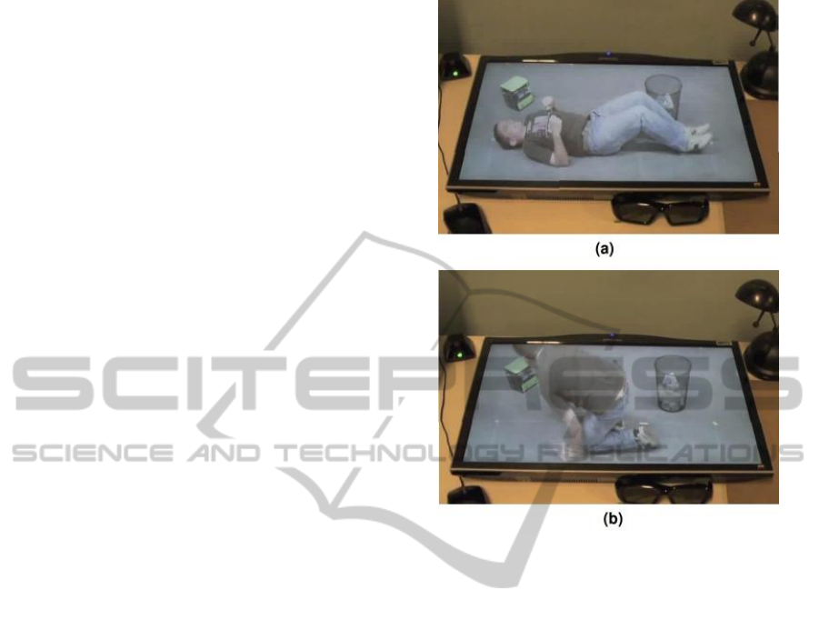
Figure 1: (a) An image that satisﬁes all requirements to pro-

duce the “Sense of Reality”. (b) An image whose border

produces a cut in the scene that affect the tridimensional

interpretation.

in a horizontal position, taking care with the scene

setup. For example, Figure 1-a illustrates a case in

which all the requirements to produce the “Sense of

Reality” are satisﬁed.

The idea of generating stereoscopic images for

being displayed in an horizontal surface is not new.

Many devices that use Computer Graphics for gen-

erating horizontal stereoscopic images have already

appeared in the scientiﬁc literature, such as presented

in (Cutler et al., 1997), (Leibe et al., 2000), (Ericsson

and Olwal, 2011) and (Hoberman et al., 2012). On the

other hand, the case of horizontal stereoscopic images

generated by Image Processing is a subject not much

discussed. Our bibliographic research shows that it

has ﬁrstly appeared in the patent literature in (Wester,

2002) and (Aubrey, 2003) in a not very formal treat-

ment. As far as we know, the ﬁrst scientiﬁc paper

that handled this problem formally is (Madeira and

Velho, 2012). This paper shows that the generation

of horizontal stereoscopic images can be interpreted

as a problem of estimation and application of homo-

graphies, and it proposes the use of Computer Vision

techniques to estimate them. It uses the establishment

VISAPP2015-InternationalConferenceonComputerVisionTheoryandApplications

532

of 3D-2D correspondences between 3D points of a

calibration pattern and their respective 2D projections

over images.

We have not found any reference about a method

for generating horizontal stereoscopic pairs without

using calibration patterns, so we decided to attack this

problem just using homologous points, giving more

ﬂexibility to the user. We solved it minimizing a mea-

sure that we call by Three-dimensional Interpretabil-

ity Error, which has a simple geometric interpretation.

We also prove that this optimization problem has four

global minima, one of which corresponds to the de-

sired solution. After that, we present techniques to

initialize the optimization process avoiding the con-

vergence to a wrong global minimum.

We have tested the method and achieved good re-

sults.

2 HOMOGRAPHIES AND

CAMERA PARAMETERS

Lets consider the problem of generating a stereo-

scopic pair designed for being presented over an hor-

izontal surface.

Suppose that there is a camera in an oblique posi-

tion capturing the projection p1 of an object over an

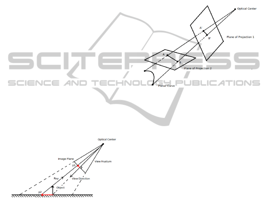
horizontal surface ( Figure 2 ). We need to ﬁnd a way

Figure 2: The rays emitted by the object and passing

through the eye have the same color as the correspondent

point in the horizontal surface.

to compute the projection p2, that corresponds to the

projection of the object using the same optical center

as the one used for capturing p1 but replacing the pro-

jective plane by the horizontal surface. It makes the

rays emitted by the object and passing through the eye

have the same color as the correspondent point in the

horizontal surface, thus the eye sees the same image

whether it came from the real object or from p2.

It is easy to notice, by examining Figure 3, that

if a set of points in a scene is projected by a cam-

era over a set of collinear projections, then they keep

collinear if we maintain the optical center in the same

place and change the position of the projection plane.

It happens because the rays whose intersection gen-

erate these projections must be coplanar, and if the

optical center is unchanged they still have to be used

for deﬁning the projections over the plane in the new

position. Since the rays are coplanar, the intersection

of them with any plane must be collinear.

Figure 3: This example shows a curve whose projection

over a projection plane is collinear. As a consequence, it

is also collinear if we change the projection plane and keep

the optical center unchanged.

This result implies that there is a homography re-

lating the coordinates of projections, measured over

the images captured by the cameras pointed to the ob-

ject to be captured, and the coordinates of the projec-

tions, made by using the same optical center as center

of projection and using the planar support as projec-

tion plane. It means that, the projections p1 and p2,

presented in Figure 2, are related by a homography.

Lets suppose that there is a 3D coordinate system

located on the horizontal plane, such that the x-axis

and y-axis are on the plane. Lets consider that the

camera used for capturing the image of the object over

the plane is deﬁned in this coordinate system by a pro-

jective transform T : RP

→ RP

given by

T = K









where K is the matrix of intrinsic parameters.

We can establish a homography H between the

horizontal plane and the image plane by restricting

the domain of T to the xy-plane. More speciﬁcally,

H = K









HorizontalStereoscopicDisplaybasedonHomologousPoints

533

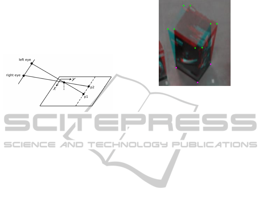
Each possible choice of x-axis and y-axis on

the horizontal plane will deﬁne a different homogra-

phy. The choices that are adequate for generating the

stereoscopic effect are the ones that will make homol-

ogous points have the same y-coordinate. It happens

when the x-axis is parallel to the line passing through

the eyes of the observer and the y-axis is orthogonal (

Figure 4 ).

Figure 4: An adequate choice of x and y axis. The x-axis

is parallel to the line passing through the eyes of the ob-

server, and the homologous points p1 and p2 have the same

y-coordinate.

This link between the camera model and homo-

graphies shows that the problem of ﬁnding the ho-

mographies appropriated for generating horizontal

stereoscopic pairs can be solved by calibrating the

camera using an adequate coordinate system over the

horizontal plane.

3 THE THREE-DIMENSIONAL

INTERPRETABILITY ERROR

It is easy to notice that any stereoscopic pair prepared

for being observed in a horizontal position must sat-

isfy the following constraints.

1. homologous points that are leveled to the horizon-

tal surface must be coincident.

2. homologous points that are not leveled to the hor-

izontal surface must have the same y-coordinate.

In order to ﬁx notation, we assume that the ho-

mologous pairs of points that correspond to 3D points

leveled to the horizontal surface are points of Type I,

and the ones that are not leveled are points of Type

II. And we also assume that the 3D point is classiﬁed

in the same group as its respective homologous pair.

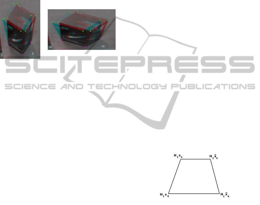
The Figure 5 illustrates the constraints related to each

type.

We deﬁne the Three-dimensional Interpretability

Error as a measure of how the constraints related to

points of Types I and II are being satisﬁed. More

precisely, lets suppose that {(p

),...,(p

)}

is a set of homologous pairs of Type I and

Figure 5: An anaglyph of a cube prepared for being pre-

sented in horizontal position. The green dots are homolo-

gous pairs of Type II. Each pair is formed by points with

the same y-coordinate. The pink dots are coincident homol-

ogous points, they are homologous pairs of Type I.

{(q

),...,(q

)} is a set of homologous pairs

of Type II. We deﬁne the Three-dimensional Inter-

pretability Error as

∑

i=1

−

+ β

∑

j=1

−

)

where α ∈ R deﬁnes the importance of the con-

straints of Type I, and β ∈ R deﬁnes the importance

of the constraints of Type II.

4 THE IMPORTANCE OF THE

INTRINSIC PARAMETERS

It is obvious that any stereoscopic pair presented

horizontally must have the Three-dimensional Inter-

pretability Error equals to zero, for any considered set

of homologous point. A non obvious question is:

If we ﬁnd homographies that make a pair of

captured images have the Three-dimensional Inter-

pretability Error equals to zero, can we assume that

the generated stereoscopic pair represents the 3D

scene correctly ?

The answer is: No. If H

and H

produce a stereo-

scopic pair with Three-dimensional Interpretability

Error equal to zero, then MH

and MH

also gener-

ate a stereoscopic pair with Three-dimensional Inter-

pretability Error equal to zero, if

M =





0 0

0 α

0 0 1





with α

∈ R − {0}, α

∈ R − {0} and α

6= α

VISAPP2015-InternationalConferenceonComputerVisionTheoryandApplications

534

As presented in Section 2, the correct estimation

of homographies corresponds to the correct calibra-

tion of the camera pair, but the possibility of assigning

and α

to different values means that the intrinsic

parameters of the camera are not well deﬁned, such

as presented in the Figure 6. It means that we cannot

calibrate the intrinsic parameters by minimizing the

Three-dimensional Interpretability Error.

Figure 6: Both pictures present stereoscopic pairs whose

Three-dimensional Interpretability Error is zero. The dif-

ference between them is the intrinsic parameters of the cam-

eras related to each applied homography.

5 FOUR GLOBAL MINIMA

In the previous section we concluded that it is not suf-

ﬁcient to ﬁnd the pair of homographies that makes the

Three-dimensional Interterpretability Error equal to

zero in order to generate the correct horizontal stereo-

scopic pair, because we can ﬁnd different results re-

lated to different choices of intrinsic parameters.

Now we present a Theorem that shows that if we

ﬁx the correct intrinsic parameters, there are just 4

different pairs of homographies that make the Three-

dimensional Interterpretability Error equal to zero. It

is important because it means that, if we know the

intrinsic parameters, and if we choose a parametriza-

tion for the cameras that ﬁx them, we can estimate

the homographies minimizing the Three-dimensional

Interterpretability Error. We just have to initiate the

optimization process sufﬁciently close to the correct

minimum in order to avoid the convergence to one of

the 3 incorrect solutions.

Theorem 1. Lets suppose that at least 4 pairs of ho-

mologous points of Type I and 2 pairs of homologous

points of Type II are known. If there is a pair of homo-

graphies H

and H

that makes the points of Type I be

coincident and that makes the points of Type II have

the same y-coordinate then, keeping the intrinsic pa-

rameters unchanged, there are exactly other 3 pairs

of homographies, deﬁned with an ambiguity of trans-

lation, that also do it. Moreover, these pairs have the

form W H

and W H

, where W can be:

1 0 ∗

0 −1 ∗

0 0 1

−1 0 ∗

0 1 ∗

0 0 1

−1 0 ∗

0 −1 ∗

0 0 1

Proof

and H

are homographies that make the homolo-

gous points satisfy their constraints. Lets suppose that

and W

also do this.

Lets suppose that {(x

), ..., (x

)} are 4 pairs

of homologous points of Type I. Since H

e H

make

the homologous points of Type I be coincident we

have that, ∃y

, ..., y

∈ RP

such that:

= H

= y

, where i ∈ {1, 2, 3, 4}. (1)

and W

also make the homologous points

of Type I be coincident thus:

= W

, where i ∈ {1, 2, 3, 4}. (2)

Since the range of 4 points by W

and W

are

equals we have, by the Fundamental Theorem of Pro-

jective Geometry, that W

= W

In order to ﬁx the notation, lets deﬁne the homog-

raphy W by:

W = W

= W

. (3)

Lets (x

) and (x

) be two pairs of homolo-

gous points of Type II.

Because H

and H

map homologous points of

Type II over points with the same y-coordinate we

have that {H

, H

} deﬁne the ver-

tices of a trapezium with two sides parallel to the x-

axis, as shown in Figure 7.

Figure 7: Trapezium whose sides deﬁned by the vertices

and H

and the side deﬁned by the vertices H

and H

are parallel to the x-axis.

Since W H

and W H

also map homologous points

of Type II over points with the same y-coordinate, it

is necessary that W maps the trapezium over other

trapezium with sides parallel to the x-axis. It means

that, ∃λ ∈ R such that

W (1, 0, 0)

= (λ, 0, 0)

. (4)

Therefore, W has the form

W =





λ a d

0 b e

0 c f





. (5)

HorizontalStereoscopicDisplaybasedonHomologousPoints

535

W H

and W H

must be homographies that cor-

respond to cameras whose intrinsic parameters are

the same as the one related to the homographies H

and H

. In other words, lets consider the vectors

t, t

∈ R

and the rotation matrices R = (r

) and

= (r

) such that

−1

= K(r

t) (6)

and

−1

= K(r

), (7)

it must exist vectors

∈ R

and rotation matrices

R = (

) and

= (

) such that

−1

= K(

t) (8)

and

−1

= K(

). (9)

Thus, we have

t) = (





λ a d

0 b e

0 c f





(10)

and

) = (

)





λ a d

0 b e

0 c f





. (11)

From the equations 10 and 11 we have

= λ

(12)

and

= λ

, (13)

from which we conclude that λ = 1 or λ = −1.

Lets consider the case λ = 1. The case λ = −1 can

be analyzed analogously. In this case we have that

(14)

and

. (15)

The vector

is orthogonal to

, as a conse-

quence, from the equation 14 we have that it is also

orthogonal to the vector r

. That means, ∃m

, m

∈ R

such that

= m

+ m

. (16)

Analogously, ∃m

, m

∈ R such that

= m

+ m

. (17)

We have that {r

, r

} is a base to R

, as well as

, r

}. So ∃k

, k

∈ R such that:

t = k

+ k

(18)

and

= k

+ k

. (19)

From the equations 10 and 11 we have

= ar

+ b(m

+ m

) + c(k

+ k

)

(20)

and

= ar

+ b(m

+ m

) + c(k

+ k

(21)

As a consequence, we have that

a + ck

= 0, (22)

a + ck

= 0, (23)

+ ck

= 1, (24)

+ ck

= 1, (25)

+ ck

= 0 (26)

and

+ ck

= 0. (27)

Now we will show that m

= 0 and m

= 0.

Lets suppose, by contradiction, that m

6= 0. From

the equations 22 and 23 we conclude that

= ck

, (28)

thus c = 0 or k

= k

If c = 0, we have from the equation 26 that b = 0,

which contradicts the equation 24, which states that

= 1.

If k

= k

then

t, r

i = k

= k

= h

, r

i. (29)

Lets assume that c

∈ R

is the optical center

of the camera related to the homography W H

, and

∈ R

is the optical center related to the homogra-

phy W H

. We have that

t, r

i = h

i = h−

i = h−c

i =

= h−c

, (1, 0, 0)

i = (−c

)

(30)

We can rewrite the equation 29 as

)

= (c

)

. (31)

Since two points of Type II are mapped over

points with the same y-coordinate, it is necessary that

)

= (c

)

and (c

)

= (c

)

, then we conclude that

= c

. (32)

Because the optical centers are equal, it follows

that the images of the stereoscopic pair captured by

the cameras must be related by a homography, which

is a contradiction with the fact that the images have

been captured by cameras whose optical centers were

located in different places. It means that m

= 0. A

similar reasoning can be used to show that m

= 0.

VISAPP2015-InternationalConferenceonComputerVisionTheoryandApplications

536

From the equations 16 and 17 we conclude that

= r

= −r

(33)

and

= r

= −r

. (34)

From the equations 12 and 13 we have, because λ

can be assigned to 1 or −1, that

= r

= −r

(35)

and

= r

= −r

. (36)

So W must have one of the following formats:





1 0 ∗

0 1 ∗

0 0 1









1 0 ∗

0 −1 ∗

0 0 1









−1 0 ∗

0 1 ∗

0 0 1









−1 0 ∗

0 −1 ∗

0 0 1





Moreover, it is clear that, if H

and H

satisfy the

constraints of point of Type I and II, then all these four

options for W make WH

and WH

also do it. Thus,

it is necessary and sufﬁcient that W takes one of these

four formats.

6 THE LEAST SQUARE

PROBLEM

Lets assume that the matrix of intrinsic parameters

K is known. In this section we deﬁne a least square

problem for ﬁnding the extrinsic parameters that min-

imize the Three-dimensional Interterpretability Error.

Lets suppose that two images I

and

are captured by a pair of cameras, and

{(u

, v

),...,(u

, v

)} is a set of points of Type I

and {(u

n+1

, v

n+1

), (u

n+2

, v

n+2

),...,(u

, v

)} is a set

of points of Type II, such that u

∈ I

and v

∈ I

Lets assume that the extrinsic parameters of the

camera used for capturing I

is R

and t

and for cap-

turing I

is R

and t

where









= (β

, β

)









and

= (δ

, δ

)

We deﬁne the objective function by

∑

i=1

−W

+ β

∑

i=n+1

−W

)

where

−1

= K









and

−1

= K









We can solve this problem using the Levenberg-

Marquardt algorithm. We ﬁnd the extrinsic parame-

ters R

, R

and t

ﬁxing the vector t

. If we did not

ﬁx t

neither t

then the value of the objective function

would reduce to zero when (t

)

→ ∞ and (t

)

→ ∞.

Besides that, by ﬁxing t

we do not reduce the gen-

erality of the solution, because we just deﬁne the po-

sition and the scale of one image of the stereoscopic

pair.

We highlight that an appropriate parametrization

of the space of rotations is required for solving this

problem. In our experiments we chose a parametriza-

tion based on an axis-angle representation.

7 FINDING THE INITIAL

PARAMETERS

We can ﬁnd the initial extrinsic parameters for the

least square problem deﬁned in the previous section

using the following process:

1. Take two samples R

and R

from the space of

rotations.

2. Use R

and R

and two pairs of homologous

points to ﬁnd the translations t

and t

We repeat this process with different choices for

and R

, and we select the extrinsic parameters

} that make the Three-dimensional Intert-

erpretability Error have the minimum value. This pro-

cess explores the fact that the space of rotation is lim-

ited, thus it can be sampled.

We must avoid getting samples R

and R

that

are too far from the expected correct solution. We

must keep in mind that, by the Theorem 1, there are 3

wrong pairs of rotations that also minimize the Three-

dimensional Interterpretability Error. Fortunately the

wrong rotations are far away from the correct ones (

180 degrees ).

In the next section we explain how to ﬁnd t

and t

using two pairs of homologous points, and assuming

that R

and R

are deﬁned.

HorizontalStereoscopicDisplaybasedonHomologousPoints

537

8 USING HOMOLOGOUS POINTS

TO FIND THE TRANSLATIONS

Lest suppose that I

and I

are images, (a, b)

∈ I

and (c, d)

∈ I

are the coordinate in pixels of the ho-

mologous points of Type I that correspond to a point

on the horizontal plane, and that (e, f )

∈ I

and

(g, h)

∈ I

are another pair of homologous points of

Type I that correspond to a point m

on the horizontal

plane.

We want to ﬁnd the vectors t = (t

, t

)

∈ R

and t’ = (t

, t

)

∈ R

that correspond to the trans-

lations used for capturing I

and I

Lets deﬁne H

and H

as the homographies that

map points with coordinates measured on the hori-

zontal surface into pixels in the images I

and I

, re-

spectively. That means

= (h

) = K









(37)

and

= (h

) = K









. (38)

We can choose any point over the horizontal plane

to be the origin of the coordinate system used for

deﬁning the camera parameters. Lets assume that m

is this point. By doing this, the point whose coor-

dinates are (0, 0)

is mapped by H

over the pixel

(a, b)

in the image I

, and is mapped by H

over the

pixel (c, d)

in the image I

. It means that

)









= λ









(39)

and

)









= λ









, (40)

where λ

, λ

∈ R are scalars that must be found.

Thus

= λ

(a, b, 1)

and

= λ

(c, d, 1)

It means that, t and t

are deﬁned up to the scale

factors λ

and λ

, because

t = K

−1

(41)

and

= K

−1

. (42)

We use the other pair of homologous points to cal-

culate λ

and λ

. Since t and t’ are deﬁned with an

ambiguity of one scale factor (Hartley and Zisserman,

2004), we just expect to calculate

Lets deﬁne

P =









(43)

as the inverse of the homography









and lets

Q =









(44)

be the inverse of the homography









It is easy to notice that P and Q can be calculated,

because we are assuming that the matrix of intrinsic

parameters K and the rotations related to each camera

are known.

We have that

−1









(45)

and

−1









. (46)

Applying the homography H

−1

over (e, f )

and

−1

over (g, h)

we must obtain the same point on

the horizontal plane. This means that, there is a scalar

∈ R such that

















= λ

















(47)

There follows from the equation in the ﬁrst line

that

, (e, f , 1)

, (g, h, 1)

. (48)

From the equation in the third line we have that

, (e, f , 1)

i =

, (g, h, 1)

i. (49)

Replacing the equation 48 in the equation 49 we

ﬁnd that



, (e, f , 1)



, (g, h, 1)



. (50)

VISAPP2015-InternationalConferenceonComputerVisionTheoryandApplications

538

9 FINDING THE SIZE OF THE

OUTPUT

We know that any calibration process performed us-

ing just the information of homologous points has an

ambiguity of scale (Hartley and Zisserman, 2004). As

a consequence, in the previous section we just could

ﬁnd homographies that generate stereoscopic pairs

with an ambiguity of size.

This problem can be solved, for example, if the

following extra information is available:

• The distance l between the optical centers of the

cameras, in both poses, used for capturing the

stereoscopic pair.

• The distance between two points m

and m

in the

horizontal plane, that correspond to two identiﬁ-

able pixels p

and p

The scale of the output must be chosen in such a

way that the ratio of the distance between p

and p

and the distance between the eyes becomes equal to

the ratio of the distance between the points m

and m

and the distance l.

For example, lets suppose that the distance l is

65m, and the distance between m

and m

is 20m.

Since the distance between the eyes of a person is

about 6.5cm, there follows that the output scale must

be chosen in such a way that that the distance between

and p

become 2cm.

If any geometric information about the scene is

available, the scale can be adjusted by a trial and error

method until a good perceptual result be achieved.

10 EXPERIMENTS WITH

SYNTHETIC DATA

We made 630 experiments in order to ﬁnd the ho-

mographies, minimizing the Three-dimensional Inter-

pretability Error, using synthetic cameras and points.

It means that the projections used were perfectly cal-

culated by the computer. The initialization method

used for the Levenberg-Marquardt algorithm was the

one described in the previous sections.

The experiments were divided into 15 groups

whose poses of the synthetic cameras used in the cal-

culation of projections were the same.

In each group, we calculated the distance between

a pair of reference homographies, found using 10

points of Type I and 10 points of Type II, and ho-

mographies calculated by using combinations with a

smaller number of points.

We know that the reference homographies were

found by a determined optimization problem, because

they were calculated using more points than the suf-

ﬁcient condition deﬁned by the Theorem 1. In order

to guarantee that the the Levenberg-Marquardt algo-

rithm converges to the correct global minimum, we

limited the rotations used in the sampling processes

of synthetic cameras and the rotations used during

the initialization of the optimization. We did this,

because we need to be conﬁdent that the sector of

the space of rotations considered contains only one

pair of cameras with Three-dimensional Interpretabil-

ity Error equals to zero.

We measured the distance between the pairs of ho-

mographies using the formula

||H

− H

|| + ||H

− H

||,

were H

and H

are the homographies that are being

compared to the references homographies H

and H

The norm considered to a matrix is its largest eigen-

value. Since the matrix representation of homogra-

phies are deﬁned up to a scale factor, we put all the

homographies in the form





∗ ∗ ∗

∗ ∗ 1





before applying the formula.

The results of the 15 experiments are presented in

the tables of the Appendix. In each table, the cells’

values are the distance between the reference homo-

graphies and the solution calculated using a different

combination of points of Type I and II deﬁned by the

cell’s position. The number of points of Type I is pre-

sented in the left of the table, and the number of points

of Type II is presented in the top.

We joined the information of all 15 tables in the

Table 1. Each cell of this table correspond to the

amount of tables from the Appendix whose corre-

spondent cell’s value is below 10

−4

, which is the

threshold chosen to consider that the the solution

agrees with the reference homographies.

We read the number of points of Type I and II in

the border of the Table 1 following the same logic of

the tables in the Appendix.

In order to analyze the Table 1 we must take into

a count that:

1. If there is a 0 in a cell, it means that any of the

15 considered solutions agrees with the reference

solution. Thus, the amount of points of Type I

and II related to the cell’s position is, probably,

not enough for making the optimization problem

well deﬁned.

2. It there is a number different from 0 in a cell, it

means that there is an agreement between a so-

lution and the reference. If this number is large,

HorizontalStereoscopicDisplaybasedonHomologousPoints

539

we can conclude that it happened in many tables,

meaning that probably the solution of the opti-

mization problem is well deﬁned for the amount

of points of Type I and II related to the cell’s po-

sition. This number can be different from 15, be-

cause a local minimum can be found, once we are

using a sparse sampling in the initialization, since

we had to solve hundreds of optimization prob-

lems.

Table 1: Each cell of this table corresponds to the amount of

tables from the Appendix whose correspondent cell’s value

is below 10

−4

, which is the threshold chosen to consider

that the the solution agrees with the reference homogra-

phies.

0 1 2 3 4 5 6

2 0 0 0 0 0 11 15

3 0 0 0 10 12 13 13

4 0 10 11 12 14 14 14

5 0 12 14 14 14 13 13

6 0 12 13 14 14 13 13

7 0 14 15 15 15 14 15

By analyzing the Table 1, we conclude that the

experimental result is in agreement with the Theorem

1. But we discover that, probably, 4 points of Type I

an 2 points of Type II is not a minimal combination

for solving the problem of ﬁnding the correct homo-

graphies by minimizing the Three-dimensional Inter-

pretability Error. Moreover, we establish the Conjec-

ture 1.

Conjecture 1. The minimal combinations of points

that make the Theorem 1 still valid are:

• 2 points of Type I and 5 points of Type II;

• 3 points of Type I and 3 points of Type II;

• 4 points of Type I and 1 point of Type II.

11 EXPERIMENT WITH REAL

IMAGES

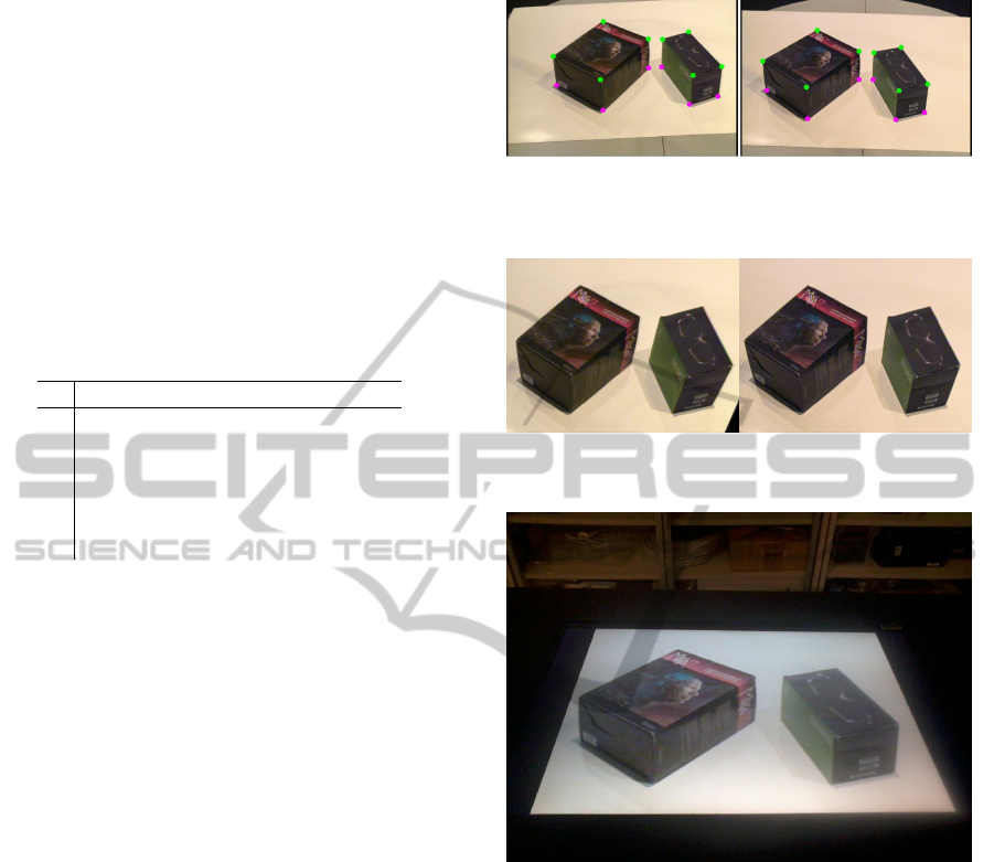
We made some experiments using real images. In Fig-

ure 8 we present a pair of images captured by two

cameras. We use colored dots to identify the homol-

ogous points used for estimating the homographies.

The pink dots correspond to points of Type I and the

green dots are points of Type II.

Figure 9 shows the stereoscopic pair generated by

the application of the homographies estimated using

the methodology described in the previous sections.

And Figure 10 shows the result presented over a hori-

zontal display. It gives the idea of the user perception

Figure 8: Two pictures used for generating an horizontal

stereoscopic pair. There are pink dots over the homologous

points of Type I, and green dots over the points of Type II.

Figure 9: Stereoscopic pair generated using the method de-

scribed in this paper.

Figure 10: One image of a stereoscopic pair being presented

over an horizontal display. This picture gives the idea of the

user perception.

( only one image of the stereoscopic pair is being pre-

sented ).

The scale of the output images was adjusted by the

user using a trial and error method.

12 CONCLUSION AND FUTURE

WORKS

We presented a new method for generating horizon-

tal stereoscopic pairs using images captured by cam-

eras. Our method is not based on the use of calibration

patterns, such as the method presented in (Madeira

and Velho, 2012). It is based on the establishment of

correspondences between homologous points, which

VISAPP2015-InternationalConferenceonComputerVisionTheoryandApplications

540

gives more ﬂexibility to the user.

An important property of our method is that

it ﬁnds the best solution considering a metric that

has an intuitive geometric interpretation, the Three-

dimensional Interpretability Error, which is deﬁned in

this paper.

We also proved a theorem that establishes a sufﬁ-

cient condition to the use of our method, and a con-

jecture that support other conditions.

Finally, we believe that this paper and (Madeira

and Velho, 2012) show that it may be possible to build

a new and interesting theory of horizontal stereoscopy

based on the deformation of images, instead of using

a rendering process. This theory would be made of re-

sults from Computer Vision, such as done in (Madeira

and Velho, 2012), or by new results, inspired in Com-

puter Vision, established using Projective Geometry

and Optimization, such as the ones presented in this

paper. Some problems that this new theory could

treats are:

1. Find good methods to initiate the Levenberg-

Marquardt algorithm that minimize the Three-

dimensional Interpretability Error.

2. Prove or disprove the Conjecure 1.

3. Find methods to estimate the 3D error of the scene

presented to the user when the capture process is

not perfect. For example, if the camera centers

are not parallel to the horizontal surface used as

reference.

4. Find the best deformation that the stereoscopic

pair must suffer in order to try to compensate the

movement of the user’s head, although this prob-

lem does not have an exact solution.

5. Deﬁne new metrics different from the Three-

dimensional Interpretability Error.

REFERENCES

Aubrey, S. (2003). Process for making stereoscopic images

which are congruent with viewer space. United States

Patent, (6,614,427).

Cutler, L. D., Fr

ohlich, B., and Hanrahan, P. (1997). Two-

handed direct manipulation on the responsive work-

bench. In Proceedings of the 1997 symposium on In-

teractive 3D graphics, I3D ’97, pages 107–114, New

York, NY, USA. ACM.

de la Rivire, J.-B. (2010). 3d multitouch: When tactile ta-

bles meet immersive visualization technologies. SIG-

GRAPH Talk.

Ericsson, F. and Olwal, A. (2011). Interaction and render-

ing techniques for handheld phantograms. In CHI ’11

Extended Abstracts on Human Factors in Computing

Systems, CHI EA ’11, pages 1339–1344, New York,

NY, USA. ACM.

Hartley, R. I. and Zisserman, A. (2004). Multiple View Ge-

ometry in Computer Vision. Cambridge University

Press, ISBN: 0521540518, second edition.

Hoberman, P., Gotsis, M., Sacher, A., Bolas, M., Turpin,

D., and Varma, R. (2012). Using the phantogram

technique for a collaborative stereoscopic multitouch

tabletop game. In Creating, Connecting and Collab-

orating through Computing (C5), 2012 10th Interna-

tional Conference on, pages 23–28.

Leibe, B., Starner, T., Ribarsky, W., Wartell, Z., Krum,

D., Weeks, J., Singletary, B., and Hodges, L. (2000).

Towards spontaneous interaction with the perceptive

workbench, a semi-immersive virtual environment.

IEEE Computer Graphics and Applications, 20:54–

65.

Madeira, B. and Velho, L. (2012). Virtual table – tele-

porter: Image processing and rendering for horizontal

stereoscopic display. In Virtual and Augmented Real-

ity (SVR), 2012 14th Symposium on, pages 1–9.

Marr, D. (1982). Vision: A Computational Investigation

into the Human Representation and Processing of Vi-

sual Information. Henry Holt and Co., Inc., New

York, NY, USA.

Wester, O. C. (2002). Anaglyph and method. United States

Patent, (6,389,236).

Yoshiki Takeoka, Takashi Miyaki, J. R. (2010). Z-touch:

A multi-touch system that detects spatial gesture near

the tabletop. SIGGRAPH Talk.

APPENDIX

There follows the 15 tables generated by the experi-

ments made using synthetic data described in the Sec-

tion 10.

Table 2.

0 1 2 3 4 5 6

2 1.4003 0.7885 0.2338 0.2883 0.2766 0.0000 0.0000

3 0.3507 0.2133 0.1625 0.0000 0.0000 0.0000 0.0000

4 0.4124 0.1775 0.2610 0.2837 0.0000 0.0000 0.0000

5 0.2216 0.0000 0.0000 0.0000 0.0000 0.0000 0.0000

6 0.1871 0.0000 0.0000 0.0000 0.0000 0.0000 0.0000

7 0.0759 0.0000 0.0000 0.0000 0.0000 0.0000 0.0000

Table 3.

0 1 2 3 4 5 6

2 0.3246 0.3358 0.1134 0.1088 0.1270 0.0000 0.0000

3 0.1132 0.1134 0.0593 0.0000 0.0000 0.0000 0.0000

4 0.0388 0.0000 0.0000 0.0000 0.0000 0.0000 0.0000

5 0.0464 0.0000 0.0000 0.0000 0.0000 0.0000 0.0000

6 0.0218 0.0000 0.0000 0.0000 0.0000 0.0000 0.0000

7 0.0718 0.0000 0.0000 0.0000 0.0000 0.0000 0.0000

Table 4.

0 1 2 3 4 5 6

2 0.4397 0.4398 0.2474 0.2468 0.2138 0.0000 0.0000

3 0.2942 0.1217 0.0953 0.0000 0.0000 0.0000 0.0000

4 0.2262 0.0000 0.0000 0.0000 0.0000 0.0000 0.0000

5 0.2652 0.0000 0.0000 0.0000 0.0000 0.0000 0.0000

6 0.2412 0.0000 0.0000 0.0000 0.0000 0.0000 0.0000

7 0.2355 0.0000 0.0000 0.0000 0.0000 0.0000 0.0000

HorizontalStereoscopicDisplaybasedonHomologousPoints

541

Table 5.

0 1 2 3 4 5 6

2 0.2615 1.0214 0.3444 0.3502 0.2016 0.0000 0.0000

3 0.1957 0.0951 0.3514 0.3514 0.0000 0.0000 0.0000

4 0.6002 0.0000 0.0000 0.0000 0.0000 0.0000 0.0000

5 0.1848 0.0000 0.0000 0.0000 0.0000 0.0000 0.0000

6 0.2007 0.0000 0.0000 0.0000 0.0000 0.0000 0.0000

7 0.1914 0.0000 0.0000 0.0000 0.0000 0.0000 0.0000

Table 6.

0 1 2 3 4 5 6

2 0.6248 0.4991 0.5126 0.5434 0.0463 0.0000 0.0000

3 0.4613 0.4961 0.6431 0.0000 0.0000 0.0000 0.0000

4 0.8455 0.4403 0.0000 0.0000 0.0000 0.0000 0.0000

5 0.4626 0.4934 0.0000 0.0000 0.0000 0.0000 0.0000

6 0.7626 0.4005 0.6388 0.0000 0.0000 0.0000 0.0000

7 0.8050 0.0000 0.0000 0.0000 0.0000 0.0000 0.0000

Table 7.

0 1 2 3 4 5 6

2 0.4310 0.4333 0.2562 0.3135 0.1940 0.5502 0.0000

3 0.3730 0.3674 0.6479 0.0000 0.0000 0.0000 0.0000

4 0.1067 0.7464 0.7723 0.0000 0.0000 0.0000 0.0000

5 0.1345 0.0000 0.0000 0.0000 0.0000 0.0000 0.0000

6 0.1487 0.7467 0.0000 0.0000 0.0000 0.0000 0.0000

7 0.1093 0.0000 0.0000 0.0000 0.0000 0.0000 0.0000

Table 8.

0 1 2 3 4 5 6

2 0.7874 0.3198 0.3140 0.3392 0.1825 0.0000 0.0000

3 0.1879 0.1711 0.7936 0.8844 0.7696 0.7654 0.6834

4 0.1550 0.0000 0.7679 0.7452 0.5967 0.6757 0.6654

5 0.5634 0.5935 0.6346 0.6295 0.4998 0.5237 0.6706

6 0.1909 0.6858 0.6874 0.6871 0.4199 0.4277 0.5338

7 0.0024 0.0000 0.0000 0.0000 0.0000 0.0000 0.0000

Table 9.

0 1 2 3 4 5 6

2 0.8925 0.4310 0.5367 0.2543 0.2095 0.0000 0.0000

3 0.2532 0.1614 0.1681 0.2341 0.3068 0.0000 0.0000

4 0.1835 0.0000 0.0000 0.0000 0.0000 0.0000 0.0000

5 0.2148 0.0000 0.0000 0.0000 0.0000 0.0000 0.0000

6 0.2102 0.0000 0.0000 0.0000 0.0000 0.0000 0.0000

7 0.1822 0.0000 0.0000 0.0000 0.0000 0.0000 0.0000

Table 10.

0 1 2 3 4 5 6

2 0.7426 0.8303 0.3292 0.3646 0.2573 0.0000 0.0000

3 0.4350 0.2784 0.5071 0.4037 0.4607 0.4367 0.4211

4 0.0307 0.0000 0.3957 0.3928 0.0000 0.0000 0.0000

5 0.2708 0.0000 0.0000 0.0000 0.0000 0.3964 0.4045

6 0.0613 0.0000 0.0000 0.0000 0.0000 0.3962 0.4069

7 0.4015 0.4405 0.0000 0.0000 0.0000 0.3949 0.0000

Table 11.

0 1 2 3 4 5 6

2 0.6068 0.3028 0.4622 0.1847 0.1440 0.0000 0.0000

3 0.4653 0.4556 0.4395 0.0000 0.0000 0.0000 0.0000

4 0.6014 0.0000 0.0000 0.0000 0.0000 0.0000 0.0000

5 0.4418 0.0000 0.0000 0.0000 0.0000 0.0000 0.0000

6 0.4010 0.0000 0.0000 0.0000 0.0000 0.0000 0.0000

7 0.4034 0.0000 0.0000 0.0000 0.0000 0.0000 0.0000

Table 12.

0 1 2 3 4 5 6

2 0.9409 0.1904 0.3584 0.2534 0.0562 0.4134 0.0000

3 0.3599 0.3445 0.3425 0.0000 0.0000 0.0000 0.0000

4 0.1694 0.0000 0.0000 0.0000 0.0000 0.0000 0.0000

5 0.2569 0.0000 0.0000 0.0000 0.0000 0.0000 0.0000

6 0.2307 0.0000 0.0000 0.0000 0.0000 0.0000 0.0000

7 0.2254 0.0000 0.0000 0.0000 0.0000 0.0000 0.0000

Table 13.

0 1 2 3 4 5 6

2 0.6323 0.8084 0.3247 0.4999 0.1544 0.3315 0.0000

3 0.3686 0.3772 0.5905 0.0000 0.0000 0.0000 0.0000

4 0.0112 0.0000 0.0000 0.0000 0.0000 0.0000 0.0000

5 0.0355 0.0000 0.0000 0.0000 0.0000 0.0000 0.0000

6 0.0395 0.0000 0.0000 0.0000 0.0000 0.0000 0.0000

7 0.0333 0.0000 0.0000 0.0000 0.0000 0.0000 0.0000

Table 14.

0 1 2 3 4 5 6

2 2.2263 0.3821 0.5053 0.2740 0.2094 0.0000 0.0000

3 0.2677 0.2671 0.2695 0.0000 0.0000 0.0000 0.0000

4 0.6059 0.4744 0.0000 0.0000 0.0000 0.0000 0.0000

5 0.0126 0.0000 0.0000 0.0000 0.0000 0.0000 0.0000

6 0.0281 0.0000 0.0000 0.0000 0.0000 0.0000 0.0000

7 0.1253 0.0000 0.0000 0.0000 0.0000 0.0000 0.0000

Table 15.

0 1 2 3 4 5 6

2 0.6504 0.4855 0.2401 0.2383 0.0609 0.0000 0.0000

3 0.0698 0.0594 0.0452 0.0000 0.0000 0.0000 0.0000

4 0.0480 0.0000 0.0000 0.0000 0.0000 0.0000 0.0000

5 0.0375 0.0000 0.0000 0.0000 0.0000 0.0000 0.0000

6 0.0739 0.0000 0.0000 0.0000 0.0000 0.0000 0.0000

7 0.0564 0.0000 0.0000 0.0000 0.0000 0.0000 0.0000

Table 16.

0 1 2 3 4 5 6

2 1.2309 0.1480 0.1603 0.1065 0.0950 0.2002 0.0000

3 0.2407 0.3813 0.1260 0.2328 0.0000 0.0000 0.0000

4 0.0807 0.2838 0.0000 0.0000 0.0000 0.0000 0.0000

5 0.4762 0.5174 0.0000 0.0000 0.0000 0.0000 0.0000

6 0.0086 0.0000 0.0000 0.0000 0.0000 0.0000 0.0000

7 0.0059 0.0000 0.0000 0.0000 0.0000 0.0000 0.0000

VISAPP2015-InternationalConferenceonComputerVisionTheoryandApplications

542