
A Rolling Shutter Compliant Method for Localisation and
Reconstruction
Gaspard Duchamp, Omar Ait-Aider, Eric Royer and Jean-Marc Lavest
Institut Pascal - COMSEE, Universite Blaise Pascal, Clermont-Ferrand, France
Keywords:
Rolling Shutter, Reconstruction.
Abstract:
Nowadays Rolling shutter CMOS cameras are embedded on a lot of devices. This type of cameras does not
have its retina exposed simultaneously but line by line. The resulting distortions affect structure from motion
methods developed for global shutter, like CCD cameras. The bundle adjustment method presented in this
paper deals with rolling shutter cameras. We use a projection model which considers pose and velocity and
need 6 more parameters for one view in comparison to the global shutter model. We propose a simplified
model which only considers distortions due to rotational speed. We compare it to the global shutter model
and the full rolling shutter one. The model does not need any condition on the inter-frame motion so it can
be applied to fully independent views, even with global shutter images equivalent to a null velocity. Results
with both synthetic and real images shows that the simplified model can be considered as a good compromise
between a correct geometrical modelling of rolling shutter effects and the reduction of the number of extra
parameters. Keywords
1 INTRODUCTION
CMOS sensors are more and more used for embed-
ded systems due to its low power consumption, low
price, and high sensitivity. Basics CMOS sensors ac-
quire image row by row, this mode allows a lighter
and faster electronic system giving a better frame rate.
The drawback is a deformation of the image due to the
relative motion camera/scene. This distortion can be a
problem when trying to catch the motion or to recon-
struct the environment when embedded on a mobile
system (Royer et al., 2007). The rise of 3D recon-
struction in urban context using cameras embedded
on cars and photos collection got from the web are
dependent on the capability of the system to deal with
such acquisitions. Different way to correct distortion
introduced by the rolling shutter or to take advantage
from them in the literature. One way is to undistort
the entire image (Liang et al., 2008), (Baker et al.,
2010), (Bradley et al., 2009). This kind of methods
gives correct visual results but is not satisfying be-
cause it does not deal with 3D structure of the scene.
(Ait-Aider et al., 2006) and (Ait-Aider et al., 2007)
solved the PNP problem of a moving object of known
geometry by taking advantage of image distortion to
get the speed of the target simultaneously with the
pose. (Meingast et al., 2005) gives a method to get
a temporal calibration of the rolling shutter, and a
correct model for small rotational speed and fronto-
parallel motion. (Magerand et al., 2012) propose a
polynomial projection model and a constrained global
optimization technique in order to solve the minimal
PNP problem without any initial guess of the solu-
tion making the method more suitable for automatic
3D-2D matching in a RANSAC framework. (Meil-
land et al., 2013) proposes a unifying model for both
motion blur and rolling shutter distorsions for dense
registration. Recently, few works adressed the prob-
lem of structure from motion using rolling shutter im-
age sequences. (Ait-Aider and Berry, 2009) studied
3D reconstruction and egomotion recovering using a
calibrated stereo rig. (Hedborg et al., 2012) presents
a bundle adjustment method which computes struc-
ture and motion from a rolling shutter video exploit-
ing the continuity of the motion across a video se-
quence. (Saurer et al., 2013) consider the stereo in the
case of a fast moving vehicle where rotational speed is
neglected and where Rolling Shutter effects are sup-
posed to be affected principally by the depth of the
scene. A recent way to handle reconstruction is not to
consider discrete poses of a camera along a trajectory,
but a continuous time motion in space as do (Ander-
son and Barfoot, 2013). Finally, (Li et al., 2013) pro-
poses an approach to correct the reconstruction using
277
Duchamp G., Ait-Aider O., Royer E. and Lavest J..
A Rolling Shutter Compliant Method for Localisation and Reconstruction.
DOI: 10.5220/0005295502770284
In Proceedings of the 10th International Conference on Computer Vision Theory and Applications (VISAPP-2015), pages 277-284
ISBN: 978-989-758-091-8
Copyright
c
2015 SCITEPRESS (Science and Technology Publications, Lda.)
inertial sensors which are more and more embedded
on devices like smartphones or notepads.
1.1 Related Work and Contribution
The closest work to ours, is the one presented in (Hed-
borg et al., 2012). Rolling shutter bundle adjustment
is achieved by exploiting the continuity of the motion
across a video sequence. A key rotation and transla-
tion is associated to the first row of each frame as in
classical bundle adjustment. In addition, the poses at-
tached to the rest of image rows are interpolated from
each pair of successive key pose parameters using
SLERP interpolation. The basic idea is to assume that
the trajectory and pose variation between frames are
smooth. The advantage of this approach is that only
six extra parameters are used for the entire sequence
in comparison to classical bundle adjustment. Never-
theless, it seems evident that the inter-frame motion
should be very small to ensure that interpolated rota-
tions and translation fit the actual values. As result,
the approach requires a high frame rate as in the ex-
periments presented in the paper. This increases the
risk of data bottleneck and/or limits the dynamic per-
formances in real time applications such as SLAM
with mobile robots. in addition, the quality of motion
estimation and triangulation is always better when the
inter-frame motion is significant. Therefore, it seems
to us that a method which estimates independent cam-
eras without any assumption about motion parameters
during inter-frame intervals is more pertinent. In the
work presented in (Saurer et al., 2013) the authors
presented a dense multi-view stereo algorithms that
solve for time of exposure and depth, even in the pres-
ence of lens distortion. The camera is supposed to
be embedded on vehicle and rotational speed is ne-
glected so that Rolling Shutter effects are supposed to
be affected principally by the depth of the scene. Un-
fortunately, as it stated in (Meilland et al., 2013) and
(Ringaby and Forss´en, 2012), in practice the lateral
rotational movements are the most significant image
deformation components, a simulation of the optical
flow is done in the paper to confirm the effect of ro-
tations and translations on rolling shutter distorsion.
In this paper we present a bundle adjustment method
to be used with rolling shutter cameras basing on the
work of (Ait-Aider et al., 2006). The approach can be
applied to totally independentviews since no assump-
tion is done on the type of motion between the cam-
eras. The speed parameters concerns only the motion
during the very short time of each frame scan-line ex-
posure. Particularly we analyze the effect of each type
of motion and propose a simplified model which con-
siders rolling shutter effects due to rotational speed
only. We make an analyse of the optical flow accord-
ing to the speed, and justify the Omission of linear
speed. This comes from the assumption that rotation
produces more significant optical flow and thus big-
ger image distortions. We make a comparative study
of 3 projection models: the classical Global Shut-
ter, the complete rolling shutter model with both rota-
tional and linear speed and the simplified rolling shut-
ter model. Results with both synthetic and real images
shows that the simplified can be considered as a good
compromise between a correct geometrical modelling
of rolling shutter effects and the reduction of the num-
ber of extra parameters.
a
b
Figure 1: Illustration of a rolling shutter effect: still cam-
era, equivalent to global shutter (a), moving rolling shutter
camera (b).
2 PROJECTION MODELS
2.1 Global Shutter
Considering the classical pinhole camera model de-
fined by its intrinsic parameters Tsai (Tsai, 1986), the
projection equation of a 3D point P = [X,Y,Z]
T
, with
VISAPP2015-InternationalConferenceonComputerVisionTheoryandApplications
278
[R T] the transformation between the object and the
camera frame is (Hartley and Zisserman, 2003):
s
˜
m = K[R − RT]
˜
P (1)
where s is an arbitrary scale factor, K the matrix
the instrinsic parameters of the camera, m = [u,v]
T
the perspective projection of P noting
˜
m,
˜
P the homo-
geneous coordinates of m,P.
2.2 Rolling Shutter
The projection equation of this point considering a
uniform motion during the time of one image scan-
ning with a rolling shutter camera is:
s
˜
m
i
= K[δR
i
R − δR
i
R(T+ δT
i
)]
˜
P
i
(2)
where τ is the delay from a line to the next one,
δR
i
is the amount of rotation due to rotational velocity
at the time corresponding to the line τ · v
i
, and δT
i
the amount of translation due to translational velocity
at this time. The index i is for the i
th
3D point, v
i
its corresponding line on the sensor and t
i
= τ· v
i
the
delay in acquisition from the first line to the line of
the current 3D point i.
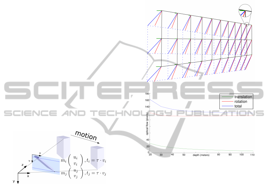
Figure 2: Perspective projection of a moving object with a
rolling shutter camera.
2.3 Simplified Rolling Shutter
Removing the linear speed from the Rolling shutter
model gives us the following projection equation:
s
˜
m
i
= K[δR
i
R − δR
i
RT]
˜
P
i
(3)
2.3.1 Optical Flow from Speed
The third model tested here is made with the assump-
tion that the rolling shutter effect due to translation is
negligible compared to the one due to rotation. The
effect induced by a linear motion parallel to the retina
is slightly the same as a rotational motion of the cam-
era according to an axe perpendicular to the linear
displacement. In the case of a frontal motion (cam-
era placed at the front or the rear of a vehicle), no
rotational motion can have the same effect and the
model with only rotational speed cannot compensate,
but in this case the optical flow consecutive to the lin-
ear motion is reduced. Fig. 3 shows the optical flow
induced by the motion of the camera. Translations
have a very lower effect and become quickly indistin-
guishable with depth of the view.
a
b
Figure 3: Simulated image of an object and the optical flow
inherent to the camera motions, green: translation (10 m/s),
red : rotation (2 rad/s), blue : both (a), optical flow ex-
pressed in pixels according to depth of the scene for each
type of motion.
3 3D RECONSTRUCTION WITH
ROLLING SHUTTER
We consider several views of a scene, each taken from
a moving rolling shutter camera. We want to get the
pose of each cam of each view and the position of 3D
points from 2D-2D detection correspondence. Previ-
ous work (Hedborg et al., 2011) considers one pose
for each line of the image, here we consider a unique
pose for each view, and the distortion is compensated
by a small motion depending of the speed and the
retina line (proportional to time since the beginning
of the acquisition). By expressing the entire system
in a single camera coordinate we get:
s
˜
n
i
= K[δR
ileft
− δR
ileft
δT
ileft
]
˜
P
i
(4)
the projection equation in the camera chosen for
being the reference.
ARollingShutterCompliantMethodforLocalisationandReconstruction
279

s
˜
n
i
= K[RδR
iright
− RδR
iright
(RδT
iright
+ T)]
˜
P
i
(5)
the projection equation for the other cameras.
We get 2N reprojection equations for each 3D
point (two in each image), each 3D point has 3 pa-
rameters and we have twelve parameters for each ad-
ditional camera pose. Thus, we need at least eigh-
teen points plus twelve per pose to solve the problem
against six plus six for the global shutter model. In
case of the simplified rolling shutter model, we only
need at least twelve points plus nine per pose.
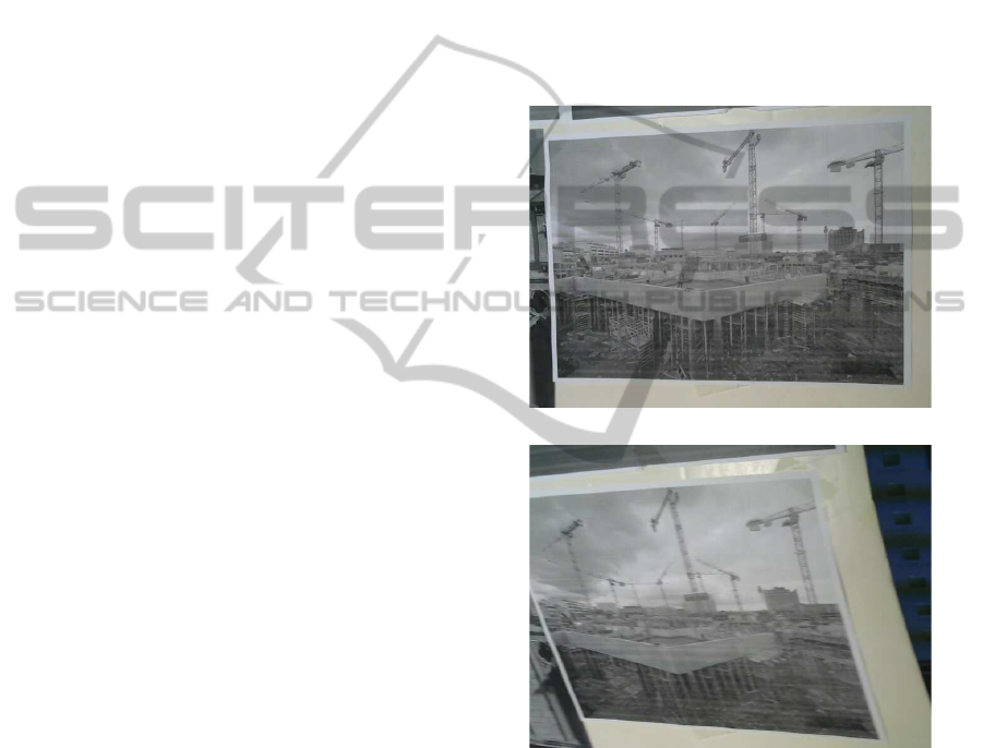
Figure 4: Two different views of a scene taken by moving
rolling shutter cameras.
This leads us to minimize the following cost func-
tion with respect to pose (R
j
,T
j
) (first camera is at
world reference), rotational speed (W
j
) and transla-
tional speed (V
j
) parameters of j
th
view:
ε(R,T,W, V) =
k
∑
j=1
l
∑
i=1
[m
ij
− p
ij
]
2
(6)
p
ij
being the detected points in j
th
image and m
ij
,
the projection in j
th
image of the 3D point P
i
associ-
ated to p
i
and q
i
.
An initial solution can be found using the epipolar
constraint. It can be more precise by adding a step af-
ter initialization; we must consider an essential matrix
per point pair instead of per image pair fig. 4.
q
T
i
E
i
p
i
= 0 (7)
With:
E
i
=
ˆ
T
i
R
i
(8)
ˆ
T
i
is the antisymmetric matrix associate to T
i
and:
R
i
= δR
T
left
RδR
right
(9)
T
i
= δR
T
left
(RδT
right
+ T− δT
left
) (10)
This leads us to a non linear system, whereas it is, for
global shutter images. In this step the linear speed is
ignored. The 3D structure is obtained by triangula-
tion.
Figure 5: Schematic view of the experimental setup with
synthetic data.
4 EXPERIMENTS
4.1 Test with Synthetic Data
4.1.1 Experimental Setup
To test the reconstruction, a first stage was to use syn-
thetic data. An object was created as a 3D point cloud.
Cameras with their own speed and pose were placed
around watching towards it. there is no correlation
between the orientation of the speed and the displace-
ment between each view. Each image of the scene is
considered as totally independent. Images were ob-
tained by application of the rolling shutter projection
equation. Resolution of the problem was then done
for each model, global shutter,rolling shutter and sim-
plified rolling shutter. The virtual object was included
in a cube of 25m edge placed at 75m to 125m from the
cameras.
Simulated cameras resolution was 1600 per 1200
pixels, the focal was 6.5mm, τ was set to 25µs. Cam-
eras speed magnitude was in range [0,10]m/s and
[0,2]rad/s for linear and angular speed. Those pa-
rameters were chosen to keep the object in the vi-
sion field and the speeds according to the ones avail-
able for a pedestrian or the autonomous vehicle VIPA
(http://www.ligier.fr/ligier-vipa). A noise on mea-
sures was applied in range [0,1]pixel, the number of
3D points in range [200,1000]points and the number
of views in range [2,10]images. All of those parame-
ters are shown in the table 1. For each set, 100 sim-
ulation were done and solved with each model. The
number of simulations is 2673000.
Fig. 6 and 7 show the loss of accuracy of the three
models according to speed.
VISAPP2015-InternationalConferenceonComputerVisionTheoryandApplications
280
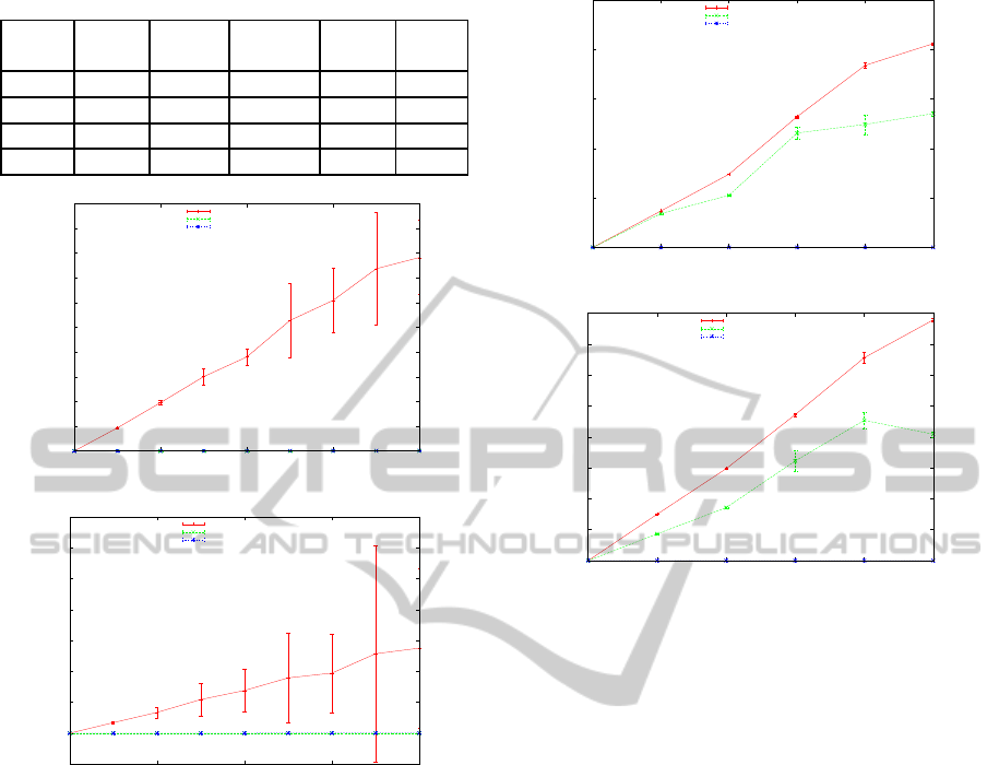
Table 1: List of parameters used for the simulation.
views 3d pts angular linear noise
speed speed
Min 2 200 0 0 0
Max 10 1000 2 10 1
Step 1 200 0.25 2 0.1
Steps 9 5 9 6 11
0
0.05
0.1
0.15
0.2
0.25
0.3
0.35
0.4
0.45
0.5
0 0.5 1 1.5 2
Error of reconstruction (m)
angular speed (rad/s)
Global Shutter
Rolling Shutter Simple
Rolling Shutter
a
-0.5
0
0.5
1
1.5
2
2.5
3
3.5
0 0.5 1 1.5 2
Error of position (m)
angular speed (rad/s)
Global Shutter
Rolling Shutter Simple
Rolling Shutter
b
Figure 6: Errors of reconstruction (a), position of cameras
(b) according to rotational speed.
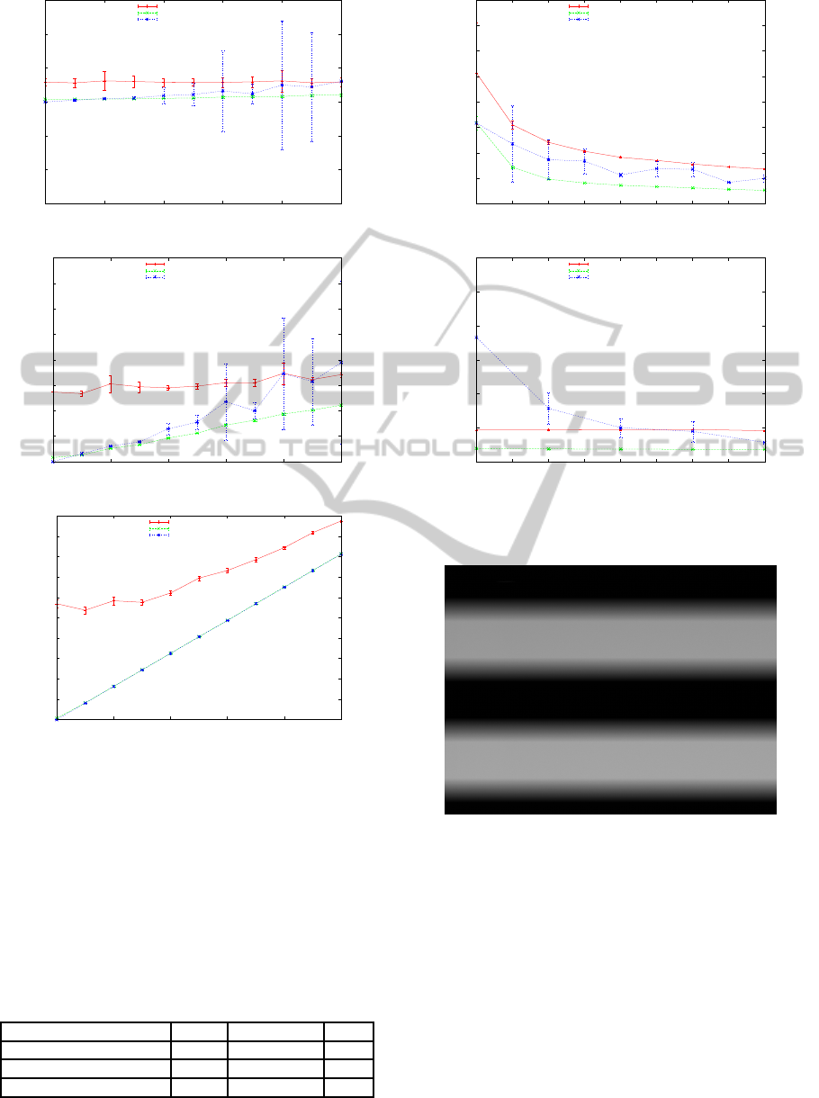
4.1.2 Noise
In this section we study robustness of the model to
noise. We added a random geometric noise follow-
ing a uniform distribution from 0 to 1 pixel every
0.1 pixel. Each measure is a mean of 100 simula-
tions following the same scheme as previously for
a speed corresponding to [10m/s, 2rad/s]. As one
can see on fig. 8, the addition of degrees of free-
dom to the system makes it less robust to noise. It
needs more views of the scene and more 3D points
to get the system constrained enough and the recon-
struction robust to a high noise level when using the
complete rolling shutter model. The simplified rolling
shutter model is more robust. Fig. 9 (a) shows the
precision of reconstruction according to the number
of cameras for a speed and noise corresponding to
[10m/s,2rad/s,0.5pixel] and 600 3D points, and (b)
0
0.005
0.01
0.015
0.02
0.025
0 2 4 6 8 10
Error of reconstruction (m)
linear speed (m/s)
Global Shutter
Rolling Shutter Simple
Rolling Shutter
a
0
0.02
0.04
0.06
0.08
0.1
0.12
0.14
0.16
0 2 4 6 8 10
Error of position (m)
linear speed (m/s)
Global Shutter
Rolling Shutter Simple
Rolling Shutter
b
Figure 7: Errors of reconstruction (a), position of cameras
(b) according to translational speed.
the precision of reconstruction according to the num-
ber of 3D points for a speed and noise corresponding
to [10m/s,2rad/s,0.5pixel] and 4 views.
4.2 Experiment with Real Data
4.2.1 Sensor Calibration of Parameter Tau
Objective removed, all the cells of the sensor are ex-
posed at the same time to a flashing light whose fre-
quency is known. The frequency of the light is high
enough regarding the rolling shutter frequency to see
several flashes. The lag between each line of the sen-
sor is deduced by a simple ration between periods of
the light signal and the number of lines it overlaps.
The time found for our camera is 110µs.
4.2.2 Reconstruction
To illustrate the relative robustness of the simplified
rolling shutter model beside the complete one, and
the gain of precision from the global shutter one, it
was tested to reconstruct a 3D structure. The chosen
structure is a corner to easily visually check if any de-
formations occurs during the reconstruction. We can
see on Fig. 11 that the reconstruction presents no ap-
parent distortions on the global structure, this is more
ARollingShutterCompliantMethodforLocalisationandReconstruction
281
-6
-4
-2
0
2
4
6
0 0.2 0.4 0.6 0.8 1
Error of position (m)
amount of noise (m/s)
Global Shutter
Rolling Shutter Simple
Rolling Shutter
a
0
0.1
0.2
0.3
0.4
0.5
0.6
0.7
0.8
0 0.2 0.4 0.6 0.8 1
Error of reconstruction (m)
amount of noise (pixel)
Global Shutter
Rolling Shutter Simple
Rolling Shutter
b
0
0.05
0.1
0.15
0.2
0.25
0.3
0.35
0.4
0.45
0.5
0 0.2 0.4 0.6 0.8 1
Error of reprojection (pixel)
amount of noise (pixel)
Global Shutter
Rolling Shutter Simple
Rolling Shutter
c
Figure 8: Errors of position of cameras (a), reconstruction
(b), reprojection (c) according to noise, with randomly ori-
ented speeds of 2rad/s.
evident to see on the attached video. The camera used
is a webcam logitech C310,used with a resolution of
640 by 480 pixels and a focal distance of 4 mm. The
final parameters of reconstruction such as the num-
ber of inlier 3D points, inlier observations, and final
reprojection error RMS are shown in table 2.
Table 2: Results of the reconstruction.
3dpts observation rms
Global Shutter 2537 10615 0.86
Rolling Shutter 3273 13204 0.84
Rolling Shutter Simple 3446 13639 0.77
0
0.1
0.2
0.3
0.4
0.5
0.6
0.7
0.8
2 3 4 5 6 7 8 9 10
Error of reconstruction (m)
number of views
Global Shutter
Rolling Shutter Simple
Rolling Shutter
a
0
0.2
0.4
0.6
0.8
1
1.2
200 300 400 500 600 700 800 900 1000
Error of reconstruction (m)
number of 3D points
Global Shutter
Rolling Shutter Simple
Rolling Shutter
b
Figure 9: Errors of reconstruction according to the number
of views (a), to the number of 3D points (b).
Figure 10: Image used for the temporal calibration of
CMOS rolling shutter sensor. Objective removed, all the
cells of the sensor are exposed at the same time to a flash-
ing LED whose frequency is controlled with a square signal
generator and an oscilloscope (Meingast et al., 2005).
5 DISCUSSION
In addition to the presentation of the simplified rolling
shutter model, the results in Fig.6 and 7 show that the
impact from linear speed on the quality of the recon-
struction is less than the one from the rotational speed
in the same way of the optical flow previously stud-
ied. As well the addition of variables to the system
VISAPP2015-InternationalConferenceonComputerVisionTheoryandApplications
282
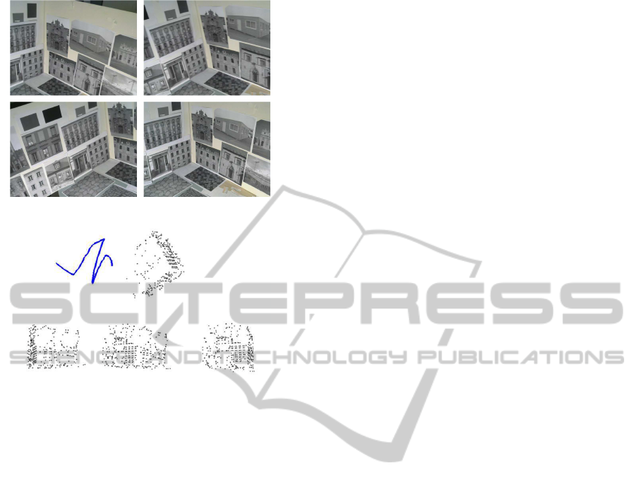
a
b
Figure 11: Motion and reconstruction of a trajectory, (a)
some images used for the reconstruction, (b) in blue the mo-
tion of the camera and in black the 3D reconstruction from
different point of view.
makes it less constrained and so cause a decay in its
robustness to noise. According to Fig. 8 and 9 the
simplified rolling shutter model is more robust than
the complete one. In addition, it is faster to solve
(less parameters to optimise, less derivation a fortiori
numerical ones, smaller jacobians). Less variables re-
duces too the probability to have local minima.
A system which doesn’t need successive se-
quences of near images allow to work with spatially
and time spaced images (leading better triangulation
due to a more pronouncedstereo), the inclusion of im-
ages taken out of the sequence both rolling and global
shutter. It results a lighter application with less pro-
cessor charge and less data transfer via the bus. Cur-
rently the methods in reconstruction are not in using
all the images from the camera but selecting them,
as seen in (Mouragnon et al., 2009). The presented
method is suitable in the actual state of art SLAM by
its spatially and temporally spaced acquisition robust-
ness.
6 CONCLUSIONS
We presented a method to deal with rolling shutter
distortion for SFM applications relevant in the cur-
rent state of art. The method is accurate thanks to
the modelling of the motion; generic, it can deal with
both rolling shutter and global shutter images; robust
thanks to the use of only very useful parameters; us-
able with very low frame rate video. We think that
this method can be very useful in many applications
in robotics, or in augmented reality applications with
the use of devices such as phones or notepads whose
embedded cameras are rolling shutter. We envisage to
use the effect of rolling shutter on primitives to get a
priori on motion and robustify matching.
ACKNOWLEDGEMENT
This work has been sponsored by the French gov-
ernment research program Investissements d’avenir
through the RobotEx Equipment of Excellence
(ANR-10-EQPX-44) and the IMobS3 Laboratory of
Excellence (ANR-10-LABX-16-01),by the European
Union and the region Auvergne through the program
L’Europe s’engage en Auvergne avec le fond eu-
ropeen de developpement regional (FEDER).
REFERENCES
Ait-Aider, O., Andreff, N., Lavest, J. M., and Martinet, P.
(2006). Simultaneous object pose and velocity com-
putation using a single view from a rolling shutter
camera. In Computer Vision–ECCV 2006, pages 56–
68. Springer.
Ait-Aider, O., Bartoli, A., and Andreff, N. (2007). Kine-
matics from lines in a single rolling shutter image.
In Computer Vision and Pattern Recognition, 2007.
CVPR’07. IEEE Conference on, pages 1–6. IEEE.
Ait-Aider, O. and Berry, F. (2009). Structure and kinemat-
ics triangulation with a rolling shutter stereo rig. In
Computer Vision, 2009 IEEE 12th International Con-
ference on, pages 1835–1840. IEEE.
Anderson, S. and Barfoot, T. D. (2013). Towards rela-
tive continuous-time slam. In Robotics and Automa-
tion (ICRA), 2013 IEEE International Conference on,
pages 1033–1040. IEEE.
Baker, S., Bennett, E., Kang, S. B., and Szeliski, R. (2010).
Removing rolling shutter wobble. In Computer Vision
and Pattern Recognition (CVPR), 2010 IEEE Confer-
ence on, pages 2392–2399. IEEE.
Bradley, D., Atcheson, B., Ihrke, I., and Heidrich, W.
(2009). Synchronization and rolling shutter com-
pensation for consumer video camera arrays. In
Computer Vision and Pattern Recognition Workshops,
ARollingShutterCompliantMethodforLocalisationandReconstruction
283

2009. CVPR Workshops 2009. IEEE Computer Soci-
ety Conference on, pages 1–8. IEEE.
Hartley, R. and Zisserman, A. (2003). Multiple view geom-
etry in computer vision. Cambridge university press.
Hedborg, J., Forss´en, P.-E., Felsberg, M., and Ringaby, E.
(2012). Rolling shutter bundle adjustment. In Com-
puter Vision and Pattern Recognition (CVPR), 2012
IEEE Conference on, pages 1434–1441. IEEE.
Hedborg, J., Ringaby, E., Forss´en, P.-E., and Felsberg, M.
(2011). Structure and motion estimation from rolling
shutter video. In Computer Vision Workshops (ICCV
Workshops), 2011 IEEE International Conference on,
pages 17–23. IEEE.
Horn, B. K. (1987). Closed-form solution of absolute orien-
tation using unit quaternions. JOSA A, 4(4):629–642.
Li, M., Kim, B. H., and Mourikis, A. I. (2013). Real-time
motion tracking on a cellphone using inertial sensing
and a rolling-shutter camera. In Robotics and Automa-
tion (ICRA), 2013 IEEE International Conference on,
pages 4712–4719. IEEE.
Liang, C.-K., Chang, L.-W., and Chen, H. H. (2008). Anal-
ysis and compensation of rolling shutter effect. Image
Processing, IEEE Transactions on, 17(8):1323–1330.
Magerand, L., Bartoli, A., Ait-Aider, O., and Pizarro, D.
(2012). Global optimization of object pose and motion
from a single rolling shutter image with automatic 2d-
3d matching. In Computer Vision–ECCV 2012, pages
456–469. Springer.
Meilland, M., Drummond, T., and Comport, A. I. (2013).
A unified rolling shutter and motion blur model for 3d
visual registration. In The IEEE International Confer-
ence on Computer Vision (ICCV).
Meingast, M., Geyer, C., and Sastry, S. (2005). Geomet-
ric models of rolling-shutter cameras. arXiv preprint
cs/0503076.
Mouragnon, E., Lhuillier, M., Dhome, M., Dekeyser, F.,
and Sayd, P. (2009). Generic and real-time structure
from motion using local bundle adjustment. Image
and Vision Computing, 27(8):1178–1193.
Ringaby, E. and Forss´en, P.-E. (2012). Efficient video rec-
tification and stabilisation for cell-phones. Interna-
tional journal of computer vision, 96(3):335–352.
Royer, E., Lhuillier, M., Dhome, M., and Lavest, J.-M.
(2007). Monocular vision for mobile robot localiza-
tion and autonomous navigation. International Jour-
nal of Computer Vision, 74(3):237–260.
Saurer, O., Koser, K., Bouguet, J.-Y., and Pollefeys, M.
(2013). Rolling shutter stereo. In The IEEE Inter-
national Conference on Computer Vision (ICCV).
Tsai, R. Y. (1986). An efficient and accurate camera calibra-
tion technique for 3d machine vision. In Proc. IEEE
Conf. on Computer Vision and Pattern Recognition,
1986.
VISAPP2015-InternationalConferenceonComputerVisionTheoryandApplications
284
