An Optimization Approach for Job-shop with Financial Constraints

In the Context of Supply Chain Scheduling Considering Payment Delay between

Members

S. Kemmoe

, D. Lamy

and N. Tchernev

CRCGM EA 3849, Université d’Auvergne, Clermont-Ferrand, France

LIMOS UMR CNRS 6158, Aubière, France

Keywords: Supply Chain, Payment Delay, Job-Shop, Linear Program, GRASP.

Abstract: In this paper the use of Job-Shop Scheduling Problem (JSSP) is addressed as a support for a supply chain

scheduling considering financial exchange between different supply chain partners. The financial exchange

is considered as the cash flow exchanges between different upstream and downstream partners. Moreover,

several suppliers are involved in operations. The problem under study can be viewed as an extension of the

classical JSSP. Machines are considered as business or logistic units with their own treasury and financial

exchanges happen between the different partners. The goal then is to propose the best schedule considering

initial cash flows in treasuries as given data. The problem is formulated as integer linear programming

model, and then a powerful GRASPxELS algorithm is developed to solve large scale instances of the

problem. The experiments on instances with financial constraints proved the methods addressed the problem

efficiently in a short amount of time, which is less than a second in average.

1 INTRODUCTION

This paper deals with Supply Chain (SC) scheduling

taking into account financial constraints. A SC

composed by individual firms is modeled. In this SC

forward flow of materials and backward flow of

cash appear. Cash flows occur over time in two

forms. Accounts Payable or cash outflows include

expenditures for the logistic activities, or equipment

and materials needed to achieve each operation.

Accounts Receivable or cash inflows are induced by

progressive payment for completed task or product.

The supply chain is modelled as a Job-shop where

each SC member is considered as a machine. The

main goal is to obtain such a schedule which

maintains during the schedule horizon a positive

cash position. Thus, a better synchronization of

material and financial flows avoiding negative cash

position leads to integration of SC performance. An

integer linear programming model is developed

where payment terms and amounts of all suppliers

and distributors are known. A GRASPxELS

algorithm, where the objective is to minimize the

completion time of all activities taking into account

the financial constraints, is proposed to solve large

scale instances.

The next section provides a brief literature review.

The section 3 introduces the assumptions used in

this study. Section 4 presents the integer linear

programming model. In section 5 a customized

GRASPxELS is presented; and the results obtained

thanks to this metaheuristic are compared with the

ones obtained with the CPLEX solver. Finally, a

conclusion and future researches are proposed.

2 RELATED WORK

Inclusion of cash flow in scheduling problem has

been studied with different objective value which

leads to the Resource Investment Problem (RIP)

(Najafi al., 2006) and the Payment Scheduling

Problem (PSP) (Ulusoy G. and Cebelli, 2000).

Depending on the objective, publications encompass

both net present value (Elmaghraby and Herroelen,

1990) and extra restrictions as bonus-penalty

structure (Russell, 1986), or discounted cash-flows

(Najafi al., 2006).

The main objective of cash manager is to have

enough cash to cover day-to-day operating expenses.

Two types of metrics are generally used to optimize

financial flow: during a given period, cash position

190

Kemmoe S., Lamy D. and Tchernev N..

An Optimization Approach for Job-shop with Financial Constraints - In the Context of Supply Chain Scheduling Considering Payment Delay between

Members.

DOI: 10.5220/0005271301900198

In Proceedings of the International Conference on Operations Research and Enterprise Systems (ICORES-2015), pages 190-198

ISBN: 978-989-758-075-8

 2015 SCITEPRESS (Science and Technology Publications, Lda.)

reveals the cash which is available and cash flow,

the cash generated. (Stadtler, 2005) proposes a study

of management on supply chain where the time

horizon relative to the operational schedule

corresponds to the financial schedule. To increase

performance, financial considerations must be done

at every production level, from planning to control,

in order to avoid bank overdraft. (Bertel et al., 2008)

proposed a mixed integer linear program to find an

optimal production plan to maximize average cash

position under a deterministic multi-factory, multi-

stage, and multi-product system, modelled as a flow

shop. A Dynamic Simple Policy (DSP) has been

proposed by (Gormley and Meade, 2007) in order to

minimise transactions costs at short terms periods of

a company and in a national or international context

where financial exchanges are not independently

distributed upon the global costs of the enterprise.

(Comelli et al., 2008) used an activity based costing

(ABC) system to link supply chain physical and cash

flows, proposing a tactical production planning

model. (Tsai, 2008) studied the influence of trade

terms, under a stochastic demand process, on cash

flow risks and showed that using trade discounts to

encourage early payment by customers increased

cash inflow risk despite an improved cash cycle.

(Grosse-Ruyken et al., 2011) plotted out that the

Cash Conversion Cycle (CCC) is a good measure of

performance considering upstream and downstream

partners in order to avoid the “domino effect”

resulting in the bankruptcy of a supplier.

The problems studied are usually considering

cash position as variables. Very few works propose

to analyse cash flow and scheduling problem as an

operational problem of cash management (Kemmoe

et al., 2011a). Moreover, (Elazouni and Gab-Allah,

2004) showed that “available scheduling techniques

produce financially non-realistic schedules”.

Recently (Kemmoe et al., 2011a) formulated the

problem so called “Job-shop with financial

constraint” (JSFC) which is defined as a Job-shop

problem with simultaneously consideration of

manufacturing specific resource requirements and

financial constraints. The inclusion of financial

considerations permits to consider the proper

coordination of production units when optimizing

the supply chain. The main goal is to obtain the

smallest duration of a given supply chain operational

planning while respecting the budget limit of each

production unit. Later (Kemmoe et al., 2012)

extended the model of (Kemmoe et al., 2011a) to

take into account the terms of payments and multiple

suppliers per operation.

In this paper the linear model proposed by

(Kemmoe et al., 2012) is improved for small and

medium size instances and a GRASPxELS

algorithm for large size instances for JSFC with

multiple suppliers per operation is developed.

3 SUPPLY CHAIN ASSUMPTIONS

3.1 Physical Flow Assumption

In this study the cash flow of a manufacturer who

acquires materials from suppliers, transforms them

into semi-finished or finished goods and sells them

to distributors, is considered. To better understand

this relationship a model of a given supply chain is

presented on Figure 1, where each product (P

) has

its own process plan which defines the product route

through the supply chain. Therefore the product will

be treated successively by a supplier unit (S

manufacturing units (MU

) and distributor (D

). This

supply chain can be modeled as a Job-shop

addressing the proper coordination between material

lots (jobs) and financial considerations.

Figure 1: Material and financial flows through the SC.

The Job-shop scheduling problem (JSSP) consists in

scheduling a set of n jobs that have to be sequenced

on m machines. Each job involves a set of machine-

operations, which must be processed in a pre-

determined order. Each operation has to be

processed on a given machine during a processing

time and no pre-emption is allowed. The JSSP

consists in finding a schedule with a minimal global

duration by managing machine disjunctions (see for

review (Jain and Meeran, 1999)). Using the

disjunctive graph (Roy and Sussmann, 1964) the

logistic activities can be modeled by vertices.

Precedence constraints between operations are

represented by an arc. Disjunctive constraints

between two logistic activities which require the

same logistic unit are modeled by an edge. An arc

has a total cost equal to the duration of the logistic

AnOptimizationApproachforJob-shopwithFinancialConstraints-IntheContextofSupplyChainScheduling

ConsideringPaymentDelaybetweenMembers

191

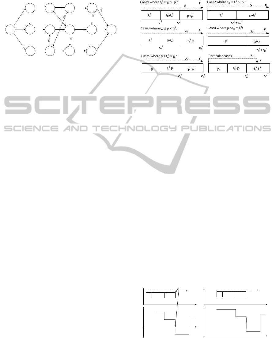
activity. The corresponding oriented disjunctive

graph of the SC problem of Figure 1is presented on

Figure 2.

Figure 2: Oriented disjunctive graph of the SC of Figure 1.

The physical flow between the manufactures is

presented at the centre of the previous graph (MU

and MU

). Since physical flows are directly

impacted by cash-flows, the assumptions concerning

cash in- and outflow are presented on the next sub-

section.

3.2 Cash Flow Assumption

The cash outflow assumption supposes that the

manufacturing units and distributors units always

pay its suppliers (suppliers or manufacturing units)

at the maturity of its accounts payable, which has a

given credit term. The cash inflow assumptions

suggest that sales/shipments occur at the end of each

processing time and that there is a given credit term

offered to customers (manufacturing units or

distributors). Using these assumptions and the

hypothesis that each activity has a known duration

and two suppliers paid with different delays, the

different events occurring during an activity can be

represented, using the following notations:

, t

: delays, respectively for the first (



) and the

second (



) suppliers, to receive financial

amount for delivering the resource

necessary to execute the corresponding

activity i.

: account receivable (financial resource or

inflow) generated by the operation i.

: starting time of activity i.

: delay between the starting time of activity i

and the time of account receivable r

: duration of material flow on activity i.

, c

: financial resource required to pay the first

and the second suppliers of the activity i.

Using these notations a set of basic examples of

events occurring during an activity is proposed in

the Figure 3. In the first case presented in the Figure

3, the supplier represented by α is paid after t

while

the second supplier represented by β is paid after t

both inside the activity. When processing time is

over, an inflow occur with amount r

after a delay δ

Figure 3: Different cash-flows events.

In the second case, two suppliers are paid at the

same time while the operation is processed. The

inflow occurs at a moment after the end of the

activity. In the third case the supplier



is paid

during the activity, while the other (



) is paid after

its end. Since the inflow occurs after a given delay,

it may happen after or before the payment of the

second supplier as presented on the fifth case. The

fourth case shows two suppliers paid at the same

time after the end of the operation. In the fifth case,

the suppliers are all paid after the end of the

operation but at different times. Finally, the sixth

case is a special one where the first supplier is paid

inside the activity but the inflow happen before the

payment of the second supplier who is paid after the

end of the activity. This case can be encountered

when an enterprise has negotiated with its supplier a

larger delay. Thanks to the income of money, the

enterprise may perhaps use this inflow for some

financial optimization involving bank interests.

The main objective during the SC scheduling is

to find a schedule which minimizes the lead time

while respecting the budget limit of each SC

member avoiding negative cash position as shown in

Figure 4.

Figure 4: Schedule of operation i with and without

negative cash position.

1,0

2,0

3,0

1,1 1,2 1,3

2,1 2,2 2,3

3,1 3,2 3,3

...

time

Cash

Position

Supplier payment conducting to a

negative cash position for operation i

Cash

Position

-t

-pi

δi

...

-t

-pi

δi

Starting time of operation i is delayed to avoid

negative cash position

ICORES2015-InternationalConferenceonOperationsResearchandEnterpriseSystems

192

In the first part of Figure 4 the supplier payment

leads to a negative cash position on the treasury

associated to the MU. In the example proposed, an

inflow occur after a given period and is important

enough to have a positive cash position. Thus, in

order to keep positive cash position when the second

supplier is paid, the starting time of activity i on MU

must be increased. This is shown on second part of

Figure 4. Concerning the cash position, it can be

seen that the shift did not affect the previous cash

flows (the first part are identical), they just happen

later in the Gantt diagram. We end up having the

following problem. We are given a set of jobs,

machines and precedence constraints between the

job operations and then we want to find a scheduling

such that at each step of the time the cash flow is

positive and the finish time is minimized.

4 LINEAR PROGRAMMING

The model presented in this section has been built to

obtain exacts solutions avoiding bank overdraft by

repartition of financial resources among the different

stakeholders. It relies on a flow added to the

incumbent Job-shop.

4.1 Parameters

Some extra parameters are taken into account and

added to those presented on the Cash flow

assumption sub-section:

M : set of logistic units;

: Job of the activity i;

V : set of all activities;

i,j : indexes representing the different activities

to schedule, i=1,..,|V|, j=1,..,|V| ;

: logistic unit required to process activity i,

∈

: initial cash flow for the logistic unit m

∈

F : set of suppliers;

f : index representing the different suppliers of

an activity, f=1,..,|F| (precedently α β);

H : a large positive number.

4.2 Variables

max

: completion date of all activities;

: starting time of activity i;

i,j

: binary variable equal to 1 if activity i is

realized before activity j and equal to 0

otherwise;

i,j,f

: binary variable equal to 1 if there is a non-

null cashflow from activity i to defray the f

supplier of activity j and equal to 0

otherwise;

i,j,f

: denotes, when two activities i and j are

performed by the same logistic unit, the

number of financial units directly

transferred from supply chain activity i to

supply chain activity j (φ

ijf

≥0 if k=μ

=μ

and

i,j,f

=0 if k≠μ

);

4.3 Linear Formulation

max

CMin

(0)

Cps





Vi 

(1)





ijji

jiVji







,/,

(2)

iij

pss 



jiJJVji





,/),(

(3)

FfjiVji

ytH

pyHxss

fjifji

ifjijiij







,,,,

)(

)1(

,,,





(4)

VjFf

mMmT













,,0

(5)

fjjji

fji

tjiFfVj

,,,

,,/,













(6)

fji

,,,









fjjji

tFfVj

,/, 









(7)

fiiji

fji

tjiFfVi

,,/, 











(8)

fiiji

fji

tFfVi

,/,













(9)

jijifji

FfVjixHy











/,,,.

,,,

(10)

jifjifji

FfVjiyH













/,,,.

,,,,

(11)

jifjifji

FfVjiy













/,,,

,,,,

(12)

jifijji

jiFfVjiyx















,/,,,1

,,,

(13)

jifji

FfVji













/,,,0

(14)

The first line (equation 0) refers to the objective of

the problem: minimizing the completion time of all

operations. Constraint (1) gives the expression of the

makespan. Constraint (2) defines the precedence

between activities occurring on the same logistic

unit. Constraint (3) ensures that precedence

constraints are respected between activities of a job.

Constraint (4) adjusts starting dates of activities

when an inflow is needed. If no inflow is needed

i,j,f

= 0), the activity j starts after the end of

operation i, if i is processed before j on the logistic

unit. If y

i,j,f

= 1

then, the solver refers to (δ

-t

j,f

) as the

AnOptimizationApproachforJob-shopwithFinancialConstraints-IntheContextofSupplyChainScheduling

ConsideringPaymentDelaybetweenMembers

193

time needed between operation i and j. Constraint

(5) avoids to exceed the initial treasury available

when allocating resources to logistic unit. Constraint

(6) ensures that the sum of cash flows from logistic

units and initial treasury is equal to the cash outflow

needed for the supplier f of activity j. Constraints (7)

is identical but take into account the case where the

logistic unit receive an inflow from itself before the

payment of a supplier. Constraint (8-9) ensures that

the sum of cash flows from the considered logistic

unit to the next ones never exceeds the inflow

resulting from its activity. Constraint (10) stipulates

that if logistic activity i occurs before activity j

=1) then a cash flow is possible from i to j. If

activity i does not come before activity j (x

=0) then

no flow is allowed between i and j. Constraints (11-

12) ensure that if there is a cash flow from i to j for

the supplier f then y

i,j,f

=1. If y

i,j,f

=0 then no flow is

possible from i to j. Constraint (13) stipulates that if

activity i occurs before activity j then no cash flows

are possible from j to any supplier of i. Constraint

(14) ensures that no flow is possible between

different logistic units, overall suppliers.

5 GRASPXELS APPROACH

5.1 GRASPxELS Principles

The GRASPxELS is a multi-start metaheuristic

based on a GRASP (Greedy Randomized Adaptive

Search Procedure (Feo et al., 1994)) extended with

an ELS (Evolutionary Local Search (Wolf and

Mertz, 2007)). The GRASPxELS, first proposed by

(Prins, 2009), helped to bring very good results in

term of quality and speed to several problems. The

association of both, GRASP and ELS, aims to

propose a better metaheuristic which will explore a

wider range of solutions. A template algorithm of

the GRASPxELS is proposed below:

Algorithm 1: GRASPxELS.

Procedure name GRASP



ELS

Begin

1. S*  Ø

2. for p := 1 to np do

3. S  Construction_Phase

4. S  Local_Seach_Phase

5. if (f(S) < f(S*)) then

6. S*  S

7. endif

8. S≔EvolutionaryLocalSearch_Phase

9. if (f(S) < f(S*)) then

10. S*  S

11. endif

12. endfor

13. return S*

end

As stressed in the Algorithm 1, a GRASPxELS is

divided into three phases: the construction phase, the

local search phase and the ELS phase. The different

specificities corresponding to those different phases

are presented in the next sub-section.

5.2 Specificities

Construction phase: As the main objective is to

propose a solution with minimal makespan, a

construction rule based on the duration of the

activities is chosen. At each construction step an

activity is randomly chosen from a list of activities

with small durations.

Local search phase: We chose to use a local

search relying on the neighborhood from (Van

Laarhoven et al., 1992). The algorithm of the local

search procedure can be found in (Kemmoe et al.,

2011b).

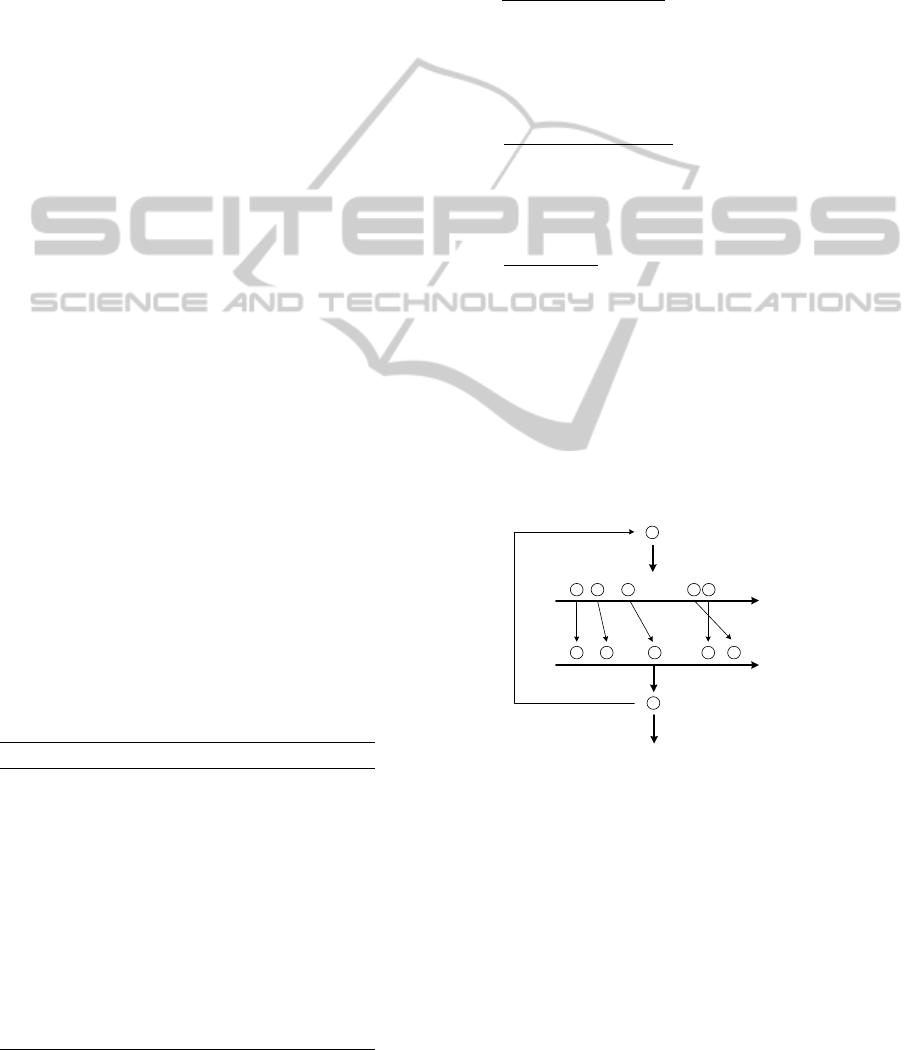
ELS phase: In the ELS phase, neighborhood of

local optimum solutions is explored through

mutations and then ameliorated thanks to the local

search. The mutation consists in permuting elements

in the repetition vector used by (Bierwirth, 1995) if

they belong to different jobs. Principles of the ELS

are shown in the Figure 5.As it can be seen in this

Figure, a neighbor could have its makespan

ameliorated or not depending on its initial quality –

this is represented with arrows between the

generation of neighbors and the local search.

...

For j from 1 to nb_ELS

Input solution

Generated

Neighbours

after LS

Best found

neighbour

Best solution

found

Higher

quality

Lower

quality

Figure 5: ELS principals.

Finally, in the next sub-section the evaluation

function for the Job-shop problem with financial

constraints is presented, as it is the most important

algorithm of this study.

5.3 Evaluation of a Bierwirth Vector

As mentioned before, a sequence of the operations

relies on a Bierwirth’s vector. The evaluation

ICORES2015-InternationalConferenceonOperationsResearchandEnterpriseSystems

194

function has been split into two parts. The first part

concerning the evaluation of the vector without cash

flows is presented in the Algorithm 2. The

Algorithm 2 returns the makespan and the starting

dates of the activities. However, no information are

given about the cash position of the treasuries.

Algorithm 2: Evaluation.

Procedure name Evaluation

Input/output



: sequence to evaluate

Input

n: number of operations

j: number of jobs

m: number of machines

Variables

i: loop index

op_M[]: last operation on machine

t_Job[]: time we have treated job

job: job treated

vertex: vertex of the job treated

machine: machine for the operation

d: end date of conjunctive predecessor

dPD: end date of disjunctive predecessor

father: predecessor

fatherD: disjunctive predecessor

Begin

1. FOR i :=0 to m DO op_M[i] = -1; END

2. FOR i :=0 to j DO t_job[i] = 0; END

3. FOR i :=0 to n DO

4. job :=



.sequence[i] ;

5. vertex := Vertex of job operation;

6. machine := machine of vertex;

7. d := 0; dPD := 0;

8. father := -1; fatherD := -1;

9. IF t_Job[job] <> 0 THEN

10. //Conjunctive father

11. father := vertex – 1 ;

12. d:= End[father];

13. END IF

14. IF (op_M[machine] <> -1) THEN

15. //Disjunctive father

16. fatherD := op_M[machine] ;

17. dPD:= End[fatherD] ;

18. END IF

19. IF (dPD > d) THEN

20. //father is the disjunctive one

21. father := fatherD ;

22. d :=dPD ;

23. END IF

24. save d and father into



;

25. Increment t_Job[job];

26. op_M[machine] ≔ vertex;

27. END

28.



.makespan:=0

29. FOR i:=0 to m DO

30. IF End[op_M[i]]> makespan THEN

31.



.makespan:= End[op_M[i]]

32. END IF

33. END

End

Consequently, another algorithm must deal with the

cash flows. The inclusion of cash flows can be done

in several ways. First the Algorithm 1 could

compute the makespan and a reparation procedure

would modify the starting dates of activities to

respect cash position of the treasuries. However this

is a bad solution because it will imply changing in

cascade in order to keep the solution consistent, thus

increasing the computation time uselessly. Hence

treasury handling must be done inside the evaluation

function with a call to the Algorithm 3 presented

below.

Algorithm 3: cashFlow.

Procedure name cashFlow

Input/Output

d: theoretic start date of operation

tr: treasury of the current machine

iT: index for moves in tables

pTr: number of negative cash position

Input

mac: current machine

del[]: suppliers delays for operation

cost[]: suppliers cost for operation

waitingP[]: awaiting inflows for tr

dInPay[]: dates of inflows for tr

Variables

dPayF: theoretic outflow date for a

supplier

f: loop index for suppliers

Begin

1. FOR f ≔1 to nbF DO

2. IF tr ≥ cost[op][f] THEN

3. disburse tr[mac] ;

4. ELSE

5. dPayF≔ d + del[op][f] ;

6. WHILE (dPayF > dInPay[mac][iT]

7. Disburse tr ;

8. Increment i_T ;

9. END

10. IF tr ≥ cost[op][f] THEN

11. Disburse tr;

12. ELSE

13. IF mac receives payment before

payment of suppliers THEN

14. collect tr;

15. END IF

16. WHILE tr < cost[op][f] AND

17. i_T < size(dInP) DO

18. collect tr;

19. d := dP[mac][i_T] – del[op][f] ;

20. I_T +=1 ;

21. END

22. Disburse tr;

23. IF tr < 0 THEN

24. Increment pTr;

25. exit(FOR) ;

26. END IF

27. END IF

28. END IF

29. END

End

The call to the Algorithm 3 in the evaluation

function is done between lines 23 and 24 of the

Algorithm 2. The important part in this algorithm is

the variable pTr as it stores the number of operations

that conduce to a negative cash position on the

AnOptimizationApproachforJob-shopwithFinancialConstraints-IntheContextofSupplyChainScheduling

ConsideringPaymentDelaybetweenMembers

195

treasury. This variable is used in a Lagrangian

relaxation-like way, keeping the solutions even if

they violate the constraint. It allows to explore non-

suited solutions that can lead to better ones while

exploring their neighborhood as it is not certain that

a direct path exists between two good solutions

without considering bad ones. Thus, if a power of

ten (PT

) directly superior to the worst possible

solution is considered, a sequence’s (seq) cost will

be formed as follows:

Seq.cost = (seq.pTr)PT

+seq.makespan

Finally, sequences are compared on their

respective costs and not on their makespan anymore.

It can be deduced from the previous formula that if

there is no problem encountered on the treasuries,

then seq.pTr = 0, and consequently seq.cost =

seq.makespan which is the wanted value. Results

obtained are presented in the next sub-section.

5.4 Computational Evaluation

The experiment is performed on twenty instances

built upon the Lawrence’s instances for the Job-shop

problem. The algorithms have been implemented in

C++ and have been executed on a 2523.09 MFLOPS

computer (Linpack Benchmark). The parameters

used in the GRASPxELS for the number of restart,

the number of ELS and the number of neighbours

are respectively 100, 50, 10. For each instance ten

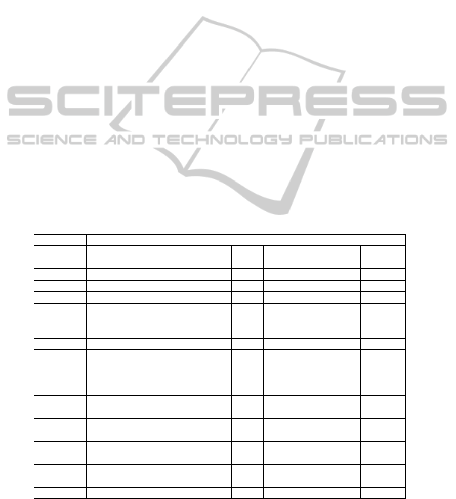
replications have been made. The results (Table 1)

are compared with the ones obtained thanks to the

linear model. On Table 1 the columns S and TT(s) of

the linear model part refer to the solutions obtain

with the CPLEX 12 solver. Concerning the

GRASPxELS part, the column S corresponds to the

average makespan, TT to the total average execution

time, TTB to the average time to the best solution,

DEV to the deviation to the best know solution

(BKS). The three other columns refer to the best

found solution (BFS), the time to found BFS and the

deviation from the BKS.

The results show the strength of the

GRASPxELS. Best solutions have been found in

less than two tenth of a second. The makespan of the

solutions are at less than 0.33 percent from the LP

BFS, and the algorithm found the optimal solution

sixteen times on the twenty instances. The presented

results show that the use of a metaheuristic is really

helpful when searching for good solutions rapidly.

Even if the results are not always the best ones, their

quality and their low deviation to the best known

solution enlighten their unavoidability when

studying large size instances.

Table 1: Results obtained with the GRASPxELS and the CPLEX solver.

Linear programming GRASPxELS

INSTANCE S TT(s) S TT TTB DEV BFS T_BFS DEV_BFS

la01

Financial

666* 176.80

666* 0.04 0.04 0 666* 0 0

la02

Financial

655* 342.26

655* 0.04 0.04 0 655* 0.01 0

la03

Financial

639* 1837.00

650.1 1.35 0.5 1.74 646 0.28 1.1

la04

Financial

615* 280.38

616.7 0.66 0.56 0.28 615* 0.35 0

la05

Financial

593* 417.07

593* 0.02 0.02 0 593* 0 0

la06

Financial

926 86400.00

926 0.01 0.01 0 926 0 0

la07

Financial

890 86400.00

890 0.02 0.02 0 890 0.01 0

la08

Financial

888 86400.00

888 2.51 0.13 0 888 0.02 0

la09

Financial

951 86400.00

951 0.07 0.07 0 951 0.01 0

la10

Financial

958 86400.00

958 0.01 0.01 0 958 0 0

la11

Financial

1222 86400.00

1222 0.03 0.03 0 1222 0.02 0

la12

Financial

1039 86400.00

1039 0.03 0.03 0 1039 0.01 0

la13

Financial

1150 86400.00

1150 0.02 0.02 0 1150 0.01 0

la14

Financial

1292 86400.00

1292 0.01 0.01 0 1292 0.01 0

la15

Financial

1216 86400.00

1207 0.09 0.09 ‐0.74 1207 0.03 ‐0.74

la16

Financial

979* 13172.13

979* 0.04 0.04 0 979* 0.01 0

la17

Financial

784* 274.01

784.6 1.85 0.82 0.08 784* 0.38 0

la18

Financial

853* 198.35

871.9 2.27 0.75 2.22 857 0.06 0.47

la19

Financial

842* 280.42

846.9 1.77 1.03 0.58 842* 0.32 0

la20

Financial

913* 301.01

934.6 2.3 0.66 2.37 927 1.11 1.53

Average :

0.66 0.24 0.33 0.13 0.12

*Asterisks denote proven optima using the LP

ICORES2015-InternationalConferenceonOperationsResearchandEnterpriseSystems

196

6 CONCLUSIONS

This study aims to present the relationship between

physical flows and cash flows through a supply

chain. The different actors of a supply chain should

carefully understand the relationship between supply

chain material activities and cash flows in order to

make operational decisions which will not

jeopardize the whole supply chain. While taking

such decisions, the goal still is to propose the highest

productivity among the supply chain. The problem is

modeled as a Job-shop scheduling problem with

financial consideration as an additional constraint. In

this study it is proposed to schedule operations or

activities while handling cash flows on treasuries in

order to always have a positive cash position. As a

consequence, the results of our study could also

affect the costs of bank overdraft that could be

negotiated. Our case study shows the relevance of

the proposed approach for a “company supply

chain”, since cash flow constraint is addressed

simultaneously with operational planning and

scheduling. Even if a mixed integer linear program

is proposed, it is difficult to solve the problem

exactly since it considers both operation scheduling

and cash-flow resolution simultaneously.

Furthermore, our instances were not representative

of the size of the problems that could be encountered

in the industry. Therefore a strong metaheuristic has

been implemented, the GRASPxELS, in order to

obtain faster results. The provided results are of

good quality, closed to the best solutions

encountered thanks to the solver which validate our

work. This study comes in addition of the past ones

on the subject of Job-shop’s like scheduling

problems with extra cash-flow constraints. A

dynamic Job-shop with random payment delays for

suppliers could be mentioned as a future study, or

the use of a flexible Job-shop model with different

payment costs depending on the chosen logistic units

for the activities.

REFERENCES

Bertel, S., Féniès, P., and Roux, O., 2008. Optimal cash

flow and operational planning in a company supply

chain. International Journal of Computer Integrated

Manufacturing, 21(4), 440-454.

Bierwirth, C. 1995. A generalized permutation approach to

Job-shop scheduling with genetic algorithms. OR

spektrum, 17, 87-92.

Comelli M., Féniès, P., and Tchernev, N., 2008.

Combined financial and physical flows evaluation for

logistic process and tactical production planning:

Application in a company supply chain. International

Journal of Production Economics, 112(1), 77-95.

Elazouni, A. and Gab-Allah, A., 2004. Finance-based

scheduling of construction projects using integer

programming, Journal of Construction Engineering

and Management ASCE 130 (1), pp. 15–24.

Elmaghraby, A. E., and Herroelen, W. S., 1990. The

scheduling of activities to maximize the net present

value of project. European Journal of Operational

Research, 49, 35-49.

Feo T. A., Resende M. G. C., Smith S. H., A greedy

randomized adaptive search procedure for maximum

independent set. Operations Research 1994;42: 860–

878.

Gormley, F. M., and Meade, N., 2007. The utility of cash

flow forecasts in the management of corporate cash

balances. European Journal of Operational Research

182, 923–935.

Grosse-Ruyken, P. T., Wagner, S. M., and Jönke, R.,

2011. What is the right cash conversion cycle for your

supply chain. Int. J. Services and Operations

Management 10, 13-29.

Jain, S., Meeran, S., 1999: Deterministic job-shop

scheduling: Past, present and future. European

Journal of Operational Research 113, 390-434.

Kemmoe, S., Lacomme, P., Tchernev, N., and Quilliot, A.,

2011a. Mathematical formulation of the Supply Chain

with cash flow per production unit modelled as job-

shop. IESM, May 25-27, Metz, France, 93-102, ISBN.

978-2-29600532-3-4.

Kemmoe, S., Lacomme, P., Tchernev, N., and Quilliot, A.,

2011b. A GRASP for supply chain optimization with

financial constraints per production unit, MIC, July

25-28, Udine, Italy.

Kemmoe, S., Lacomme, P., Tchernev, N., 2012.

Application of job-shop model for supply chain

optimization considering payment delay between

members. ILS, August 26-29, Quebec (Canada).

Najafi, A. A., Taghi, S., and Niaki, A., 2006. A genetic

algorithm for resource investment problem with

discounted cash flow. Applied Mathematics and

Computation, 183:1057-1070.

Prins, C., 2009. A GRASP x evolutionary local search

hybrid for the vehicle routing problem. In: Pereira FB,

Tavares J, editors. Bio-inspired algorithms for the

vehicle routing problem, Studies in computational

intelligence, 161, 35–53.

Roy, B., Sussmann, B., 1964. Les problèmes

d’ordonnancement avec contraintes disjonctives. Note

DS no. 9 bis, SEMA, Paris.

Russell, A. R., 1986. A comparison of heuristics for

scheduling projects with cash flows and resource

restriction. Management Science, 32(10):1291-1300.

Stadtler, H., 2005. Supply chain management and

advanced planning––basics, overview and challenges,

European Journal of Operational Research, 163(3),

575-588.

Tsai, C. Y., 2008. On supply chain cash flow risks.

Decision Support Systems 44, 1031–1042.

AnOptimizationApproachforJob-shopwithFinancialConstraints-IntheContextofSupplyChainScheduling

ConsideringPaymentDelaybetweenMembers

197

Ulusoy, G., and Cebelli, S., 2000. An equitable approach

to the payment scheduling problem in project

management. European Journal of Operational

Research, 127,262-278.

Van Laarhoven, P. J. M., Aarts, E. H. L. and Lenstra, J.

K., 1992: Job-shop scheduling by simulated annealing;

Operations Research; 40(1), 113-125.

Wolf, S., Merz, P., 2007. Evolutionary local search for the

super-peer selection problem and the p-hub median

problem. In: Lecture notes in computer science.

Berlin: Springer, 4771, 1–15.

ICORES2015-InternationalConferenceonOperationsResearchandEnterpriseSystems

198