Automatic Color-to-Gray Conversion for Digital Images
in Gradient Domain
Lu Hao, Jie Feng and Bingfeng Zhou
Institute of Computer Science and Technology, Peking University, Beijing, P.R.China
Keywords:
Color Removal, Gradient Domain, Image Processing, Color Difference.
Abstract:
Color-to-grayscale conversion for digital color images is widely used in many applications. In this paper an
automatic gradient domain color-to-gray conversion method is described. By enhancing the luminance gra-
dient with a modulated chromatic difference enhancement in CIELAB space, a gradient field is created to
construct the resulting grayscale image using a Poisson equation solver. A sign function for the gradient is
defined for isoluminance color images to keep correct color ordering. By introducing a structural similarity
index measurement (SSIM), the main parameters of the method are automatically optimized in the sense of hu-
man vision. Therefore, this method can automatically produce artifact-free and salience-preserving grayscale
images that coincide with human perception for the color difference.
1 INTRODUCTION
Grayscale images are necessary in many application
areas such as black-and-white printing, computational
photography, video and animation, etc. Hence, con-
verting digital color images into grayscale images
without losing of details and distortions in human
vision is an important issue in computer graphics.
Although some color-to-grayscale conversion algo-
rithms have been successfully used in industry, there
are still many problems remain unsolved, e.g. main-
taining the color discriminability for isoluminant col-
ors during the conversion.
In the existing literatures, there are mainly three
categories of color-to-gray conversion algorithms:
(1) Linear combination of the original color chan-
nels, typically, the Y component of CIEXYZ system
(Ohta and Robertson, 2005). This kind of algorithms
are widely used in industry, but they lack the discrim-
inability of isoluminance colors.
(2) Global optimization algorithms (Gooch et al.,
2005; Kim et al., 2009) try to avoid the problem of
category 1, by solving a global optimization problem
to modulate the final grayscale representation. How-
ever, many of this kind of methods are very time-
consuming. Some new researches introduce simpli-
This work is partially supported by NSFC grants
#61170206, #61370112, and Specialized Research
Fund for the Doctoral Program of Higher Education
#20110001110077.
fied methods to improve the computational perfor-
mance (Lu et al., 2012b).
(3) Local feature enhancement algorithms (Neu-
mann et al., 2007; Smith et al., 2008; Grundland and
Dodgson, 2007; Ancuti et al., 2011) locally enhance
the grayscale to preserve the original color and lumi-
nance contrasts, but still suffer from the low execution
efficiency and the grayscale distortion.
For an ideal color-to-gray conversion algorithm,
several requirements should be satisfied. First, the re-
sulting grayscale image have to coincide with the lu-
minance vision of human eyes, which is typically de-
fined by the L component of CIELAB
1
color model
(Wyszecki and Stiles, 1982). Second, for an isolumi-
nance color image, all the colors in the image must be
discriminable in the resulting grayscale image. Third,
no artifacts should be introduced into the resulting
grayscale image. For an image generated by a Poisson
Equation Solver (PES) working in gradient domain,
these artifacts usually appears in the form of “halo ef-
fect”, which must be reduced to be invisible by human
eyes (Fattal et al., 2002).
In this paper, we present a new category 3 algo-
rithm based on our previous work (Zhou and Feng,
2012). The new method automatically generates
grayscale images from color images under a structural
1
For simplicity, in this paper, CIELAB refers to CIE
1976 (L
∗
a
∗
b
∗
)-Space, and variables a and b are used to
stand for a
∗
and b
∗
respectively.
231
Hao L., Feng J. and Zhou B..
Automatic Color-to-Gray Conversion for Digital Images in Gradient Domain.
DOI: 10.5220/0005262102310238
In Proceedings of the 10th International Conference on Computer Graphics Theory and Applications (GRAPP-2015), pages 231-238
ISBN: 978-989-758-087-1
Copyright
c
 2015 SCITEPRESS (Science and Technology Publications, Lda.)

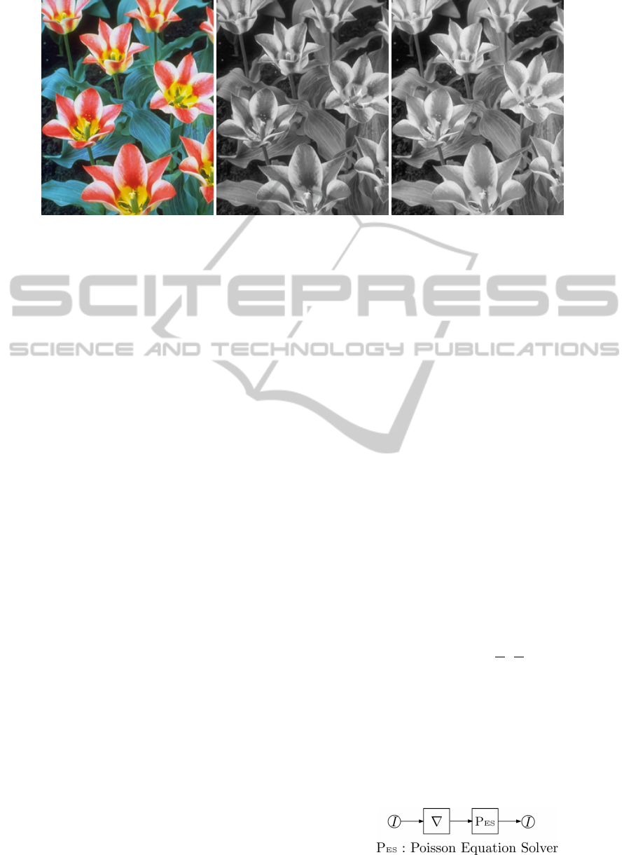
Figure 1: Gradient-domain salience-preserving color-to-gray conversion. Left: Original color image. Middle: Grayscale
image converted by our method (β = 0.2, γ = ∞,α = 0.1). Right: L in CIELAB.
similarity constrain. It performs color-to-gray conver-
sion in the CIELAB color space, and taking advantage
of the gradient domain of the image.
In gradient domain image processing, an image
can be presented by the gradients at each pixel, and
the gradient can be treated as a partial derivative of the
original image. When this partial derivative is solved
by a PDE solver such as PES, the original image can
be reconstructed. By modifying data in the gradient
domain, a different image can be obtained for certain
purpose. In Fattal’method (Fattal et al., 2002), this
strategy is used to convert a HDR image into a LDR
one, so that it can be correctly displayed in a LDR de-
vice. Similar applications can also be found in the
literature (P
´
erez et al., 2003; McCann and Pollard,
2008).
Therefore, in our method, we generate such a gra-
dient field and employs a PDE solver to reconstruct
the grayscale image from the color image. The gra-
dient at each pixel measures the color differences be-
tween its neighbors. By enhancing the luminance dif-
ference with the chromatic difference component in
CIELAB space, the salience of the original color im-
age caused by color vision can be well preserved in
the resulting grayscale image (Fig. 1). By attenuat-
ing the amount of the chromatic difference compo-
nent, grayscale distortions can be minimized and be-
come imperceptible to human eyes. Additionally, a
sign function for the color difference is also defined
to keep correct color ordering for isoluminance color
images.
This color difference is calculated base on the
CIELAB model (Ohta and Robertson, 2005), which is
a reflection of the color vision of human eyes, hence
the converted grayscale image will be an excellent
approximation of the original color image. Further-
more, there are four parameters used for attenuat-
ing the chromatic difference and keeping the color
ordering. They are automatically optimized utiliz-
ing a structural similarity index measurement (SSIM)
(Wang et al., 2004) between the converted grayscale
image and the original color image, which leads to
better preserving of the structural details of the im-
age. Experiments show that our method can produce
outstanding results in contrast to the prior works.
2 COLOR-TO-GRAY
CONVERSION IN
CIELAB-BASED GRADIENT
DOMAIN
2.1 Gradient Domain Image Processing
In gradient domain, a grayscale image I is a dis-
cretization of a continuous 2D function I(x,y) defined
in R
2
. It can be represented by the gradient ∇I of the
original I(x,y)
∇I = (I
x
,I
y
) = (
∂I
∂x
,
∂I
∂y
). (1)
The discrete form of Eq.(1) is formulated as
∇I = (I
x
,I
y
)
= (I(x + ∆x, y) −I(x,y),I(x,y + ∆y)− I(x,y)).
(2)
Therefore, this equation can be solved by a PDE
solver such as Poisson equation solver (PES) (Fattal
Figure 2: Gradient domain image processing.
GRAPP2015-InternationalConferenceonComputerGraphicsTheoryandApplications
232

et al., 2002; Press et al., 1992) to reconstruct the orig-
inal image I, as illustrated in Fig. 2. For the problem
of color-to-gray conversion, if I refers to the lumi-
nance component L of a color image C, then from the
gradient field ∇I we can reconstruct the luminance of
C (Fig. 3(d)).
(a) (b) (c) (d)
Figure 3: Color-to-gray conversion by enhancing the lumi-
nance difference with the chromatic color difference. (a)
Original color image. (b) Using chromatic difference en-
hancement without attenuation (β = 1, γ = ∞, α = 0). (c)
Artifacts removed by using attenuated chromatic difference
(β = 1, γ =
1
21
, α = 0). (d) No chromatic difference added
(β = 0, α = 0).
2.2 The Measurement of Color
Difference
CIELAB is a uniform color space, which means:
given two points in CIELAB space, their Euclidean
distance exactly measures the perceptive feeling of
color difference in human eyes for the two colors they
represent (Ohta and Robertson, 2005; Shevell, 2003).
Therefore, the color difference ∆E of the two colors
is defined by:
∆E =
q
(∆L)
2
+ (∆a)
2
+ (∆b)
2
. (3)
where ∆L, ∆a, ∆b are the differences along the co-
ordinate axis. Hence, if we use only the luminance
component L to reconstruct the grayscale image, the
resulting image will not coincide with the color differ-
ence that human eyes perceive (Gooch et al., 2005).
It is straightforward to use the color difference
in Eq.(3) which includes chromatic difference for in-
stead in constructing the gradient field. Experiments
show that more color difference can be successfully
preserved in this way (Fig. 1). However, perceptible
grayscale distortion may occur at the same time, es-
pecially where strong or noisy color differences exists
(Fig. 3(b)). In order to remove these artifacts, we add
an attenuation function A(·) to Eq.(3), whose details
will be given in Section 3. Then, the modulated color
difference is formulated as
∆E =
s
(∆L)
2
+

A

q
(∆a)
2
+ (∆b)
2

2
, (4)
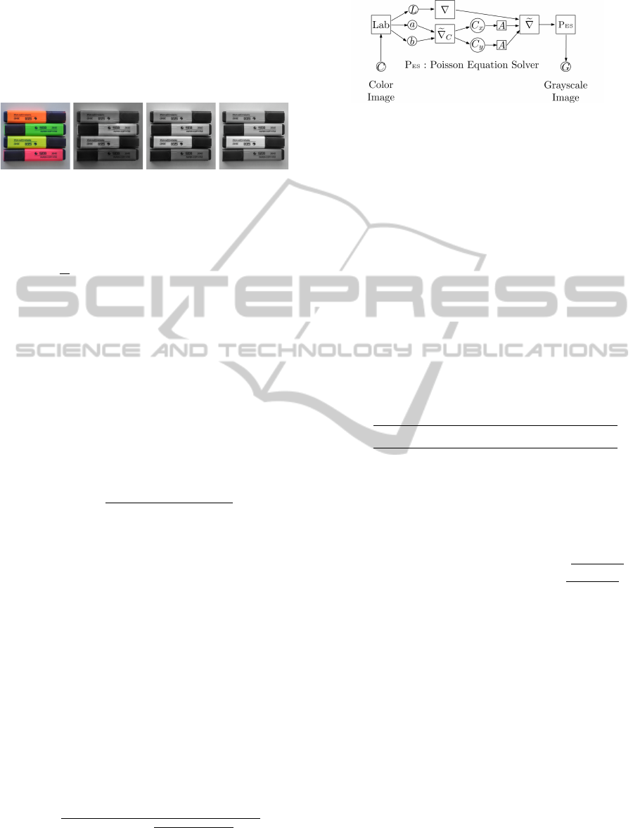
Figure 4: Color-to-gray conversion based on color differ-
ence.
2.3 Color-difference-Based
Color-to-Gray Conversion
Based on the idea of Section 2.2, we propose a new
framework that introduces chromatic color difference
into color-to-gray conversion. As shown in Fig. 4, the
input color image C is represented in L(x,y), a(x,y),
b(x,y) channels of CIELAB model. Its gradient field
e
∇C is composed of a luminance gradient component
∇L and a chromatic gradient component
e
∇
C
(a,b).
The former is calculated as in Eq.(2), and the latter
is obtained by:
e
∇
C
(a,b) = (C
x
,C
y
), (5)
where,
C
x
=
q
(a(x + ∆x, y) − a(x,y))
2
+ (b(x + ∆x, y) − b(x, y))
2
,
C
y
=
q
(a(x,y + ∆y) − a(x,y))
2
+ (b(x,y + ∆y) − b(x, y))
2
.
(6)
Then,
e
∇C can be calculated from ∇L and
e
∇
C
(a,b) us-
ing Eq.(7), before it is fed into the PES to reconstruct
the grayscale image G:
e
∇C =

sign(L
x
,a(x + ∆x, y), a(x, y), b(x + ∆x,y),b(x,y)) ·
p
L
2
x
+ A
2
(C
x
),
sign(L
y
,a(x,y + ∆y), a(x, y), b(x, y + ∆y),b(x,y)) ·
q
L
2
y
+ A
2
(C
y
)

.
(7)
Here, A(·) is the attenuation function for the chro-
matic differences C
x
and C
y
, used to remove grayscale
distortions caused by the PES. Function sign(·) de-
fines the sign of the gradient. It is used to deter-
mine the color ordering for isoluminance color im-
ages (Section 4).
3 ARTIFACT REMOVAL
When creating new images with PES, a common
problem is the existence of artifacts. In color-
to-grayscale conversion, the artifacts lead to the
grayscale distortion as shown in Fig. 3(b). There
are many works aim to solve this problem, e.g. Fat-
tal (Fattal et al., 2002) employs a multi-scale schema
AutomaticColor-to-GrayConversionforDigitalImagesinGradientDomain
233

and Neumann (Neumann et al., 2007) removes the in-
consistency of the gradient field. In our method, we
employ a single-scale method and selectively attenu-
ate the gradient enhancement to the chromatic differ-
ences to remove the artifacts. Experiments show that
this scheme is fast and efficient (Fig. 3(c)).
The attenuation of gradient enhancement takes the
form of a attenuation function A(·) as mentioned in
Section 2.2, which is defined as:
A(x) = x ·

β

1 −

x
cx
max

γ

= x · A
0
(x), (8)
where, x ∈ [0,x
max
],c ∈ [1,∞), β ∈ [0,∞) and γ ∈
(0,∞). The function works only on chromatic dif-
ference C
x
and C
y
, therefore the enhancement to the
luminance difference is always valid. Function A(·)
scales down the input signal x by a scaling function
A
0
(x). As illustrated in Fig. 5, larger value of γ
will preserve more high chromatic differences, while
smaller γ will attenuate the high chromatic difference
and preserve low chromatic differences. The constant
c is used to ensure that the largest chromatic differ-
ence will not be completely scaled down. In our im-
plementation, we choose c = 2.0. Here β and γ are
two key parameters to reduce grayscale distortions.
Their values are automatically optimized according
to a structural similarity function which measures the
degree of distortion (Section 5).
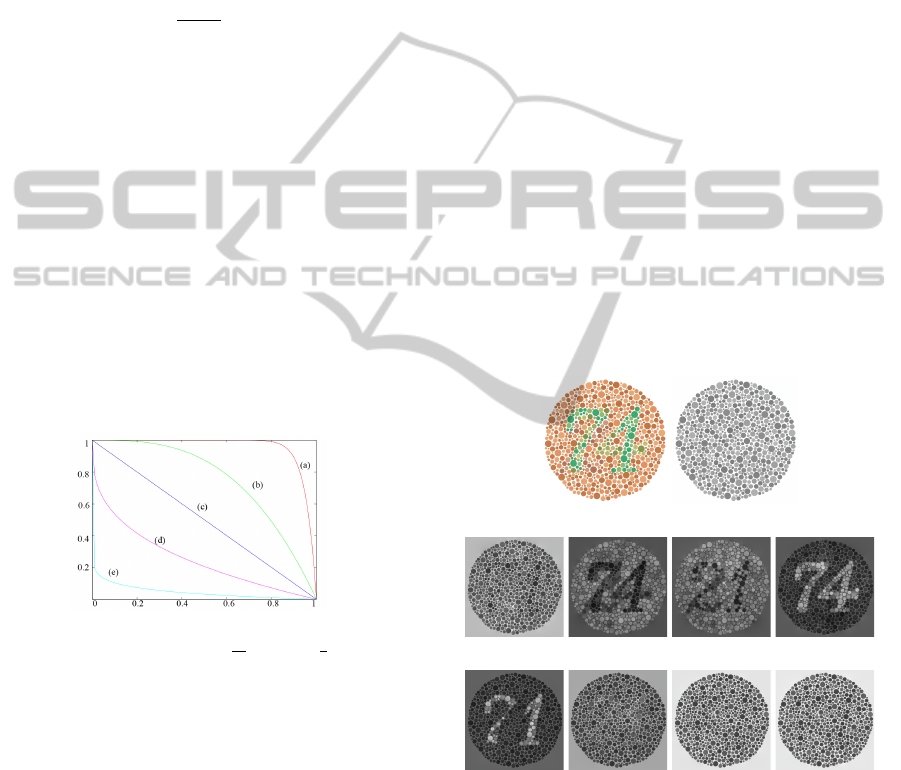
Figure 5: Image of the scaling function A
0
(x) in Eq.(8).
Here: c = x
max
= 1 and (a):γ =
1
21
, (b):γ =
1
3
, (c):γ = 1,
(d):γ = 3, (e):γ = 21.
4 COLOR ORDERING FOR
ISOLUMINANCE IMAGE
Keeping correct ordering for isoluminance colors is a
challenge for color-to-gray conversion. In a converted
grayscale image, the difference between the colors
with different luminance are easier to preserve. How-
ever, it is difficult for isoluminance colors, since they
are not discriminable in luminance. In our method,
we determine the color orders by defining a sign func-
tion for the gradient field
e
∇C.
e
∇C is constructed from the modulated color dif-
ference (Eq.(4)), hence it is not a signed value by it-
self. If there is luminance difference between a pixel
and its neighbor, the sign of the gradient at that pixel
can be reasonably defined as the sign of the lumi-
nance difference. But that do not work for a pixel that
has equal luminance with its neighbors. Instead, we
employ a similar schema as Gooch’s method (Gooch
et al., 2005). By competing the luminance difference
∆L with the chromatic difference
~
∆
C
, our sign func-
tion is defined as:
sign(∆L,a
2
,a
1
,b
2
,b
1
) = sign(∆L+α·(~v
θ
·
~
∆
C
)), (9)
where, (L
1
,a
1
,b
1
),(L
2
,a
2
,b
2
) are CIELAB coordi-
nates of two colors, ∆L = L
2
− L
1
, ~v
θ
= (cosθ,sin θ),
and
~
∆
C
= (a
2
− a
1
,b
2
− b
1
). α ∈ [0,1] defines the
strength of the chromatic difference affecting the sign
of the gradient , and θ ∈ [0,2π) defines a direction in
a-b plane of CIELAB space.
Fig. 6 demostrates the effect of our sign func-
tion. In the original image (Fig. 6(a)), the chro-
matic color differences between neighboring pixels
are larger then their luminance difference, hence the
sign function helps to reveal the color-blindness test-
ing patterns in the converted grayscale images.
(a) Original (b) L in CIELAB
(c) θ = 0
◦
(d) θ = 45
◦
(e) θ = 90
◦
(f) θ = 135
◦
(g) θ = 180
◦
(h) θ = 225
◦
(i) θ = 270
◦
(j) θ = 315
◦
Figure 6: Color discriminability testing on a color blindness
testing chart (Ishihara, 1917). Different θ reveals different
patterns (α = 1,β = 1, γ = ∞).
5 AUTOMATIC PARAMETER
OPTIMIZATION
Our color-to-gray method are able to produce perfect
GRAPP2015-InternationalConferenceonComputerGraphicsTheoryandApplications
234

salience-preserving grayscale images. Preliminary re-
sults prove the validity of our method (Fig.7). How-
ever, inappropriate parameters will result in grayscale
distortions in the converted image. In order to bet-
ter coincide with the human vision of color difference
and reduce artifacts, the four key parameters in our al-
gorithm, α, β, γ and θ, are automatically decided ac-
cording to a Structural Similarity Index Measurement
(SSIM) between the converted image and the input
image.
SSIM is a useful method for measuring percep-
tual difference between two grayscale images (Wang
et al., 2004). It considers the structural information
of an image as a feature independent of the average
luminance and contrast. To measure the similarity of
image X and Y , SSIM is defined as
SSIM(X,Y ) = [l(X ,Y )]
k
1
· [c(X ,Y )]
k
2
· [s(X ,Y )]
k
3
,
(10)
in which l(X,Y ), c(X ,Y ) and s(X,Y ) are the lumi-
nance comparison, the contrast comparison and the
structure comparison, respectively. SSIM works on an
11 × 11 window (X
j
, Y
j
), which moves over the two
images X and Y . Finally, a Mean Structural Similarity
Index Measurement (MSSIM) (Wang et al., 2004) is
calculated as the similarity of the two images:
MSSIM(X,Y ) =
1
M
M
∑
j=1
SSIM(X
j
,Y
j
). (11)
Here we extend the MSSIM to measure the sim-
ilarity of two RGB color images, by computing the
average MSSIM value of the three channels. Since
a grayscale image is also a degenerated RGB image
with equal values in the three channels, we can em-
ploy Eq.(12) to measure the similarity between the
input color image and the converted grayscale image.
MSSIM =
1
3
(MSSIM
r
+ MSSIM
g
+ MSSIM
b
) (12)
Then, by solving an optimizing problem, we can
find a group of optimal parameters
ˆ
α,
ˆ
β,
ˆ
γ and
ˆ
θ
that produce the maximum measurement value of
MSSIM:
(
ˆ
α,
ˆ
β,
ˆ
γ,
ˆ
θ) = argmax MSSIM(C, G(α, β,γ,θ)). (13)
This optimizing problem is solved by a commonly
used multi-dimension downhill simplex method
(Press et al., 1992).
From Fig. 7 we can see that the converted re-
sults with excessive enhancement of details (Column
2) turn out to have lower MSSIM values than our
optimized results (Column 3). That is because, the
grayscale distortions will affect the structural features
Original Interactive Optimized
MSSIM=1 MSSIM=0.6136 MSSIM=0.6961
β = 1, γ = 1/109 β = 2, γ = 37/26
α = 1, θ = 150
◦
α = 0.2, θ = 189
◦
MSSIM=1 MSSIM=0.6737 MSSIM=0.7888
β = 1, γ = 1/11 β = 0.1, γ = 10/11
α = 0.15, θ = 75
◦
α = 0.1, θ = 246
◦
Figure 7: Gray-scale images converted by our method. Col-
umn 2: Interactively chosen parameters excessively en-
hance the details and result in lower MSSIM; Column 3:
Automatically optimized parameters obtain higher MSSIM
and visually better results.
Table 1: Corresponding parameters of our method for Fig.
8, where columns labeled (1) through (6) correspond to the
images from left to right.
Image
Number
(1) (2) (3) (4) (5) (6)
β 0.11 0.2 0.1 0.2 0.3 0.1
γ
2
7
3
26
12
33
1
19
36
4
9
α 0.12 0.2 0.1 0.2 0.3 0.2
θ 318
◦
314
◦
230
◦
189
◦
308
◦
221
◦
of the converted images, and our extended MSSIM
has the ability of detecting these distortions and main-
taining structural similarity. Hence, it helps to find
better parameters for color-to-gray conversion.
6 EXPERIMENTAL RESULTS
We implemented our gradient domain color-to-gray
conversion method and perform it on a number of
RGB images. Input images are first converted to
CIEXYZ and then to CIELAB. The RGB color is in
PAL-RGB standard and reference white is D
65
(Ohta
and Robertson, 2005; Pascale, 2003). After the L
channel of the grayscale image is reconstructed, it
is converted back into RGB color, with the dynamic
range scaled to [0,255], and the chrominance value of
all the pixels set as that of D
65
.
In order to evaluate the quality of our method, we
compared it with 7 prior works (Lu et al., 2012a; Kim
AutomaticColor-to-GrayConversionforDigitalImagesinGradientDomain
235

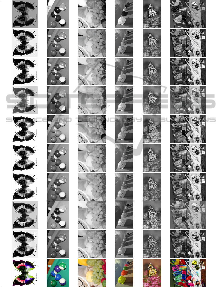
Original Ours Lu et al., CIE Y Kim et al., Grundland, Gooch et al., Neumann et al., Smith et al., Rasche et al.,
2012a 2009 2007 2005 2007 2008 2005
MSSIM 0.8224 0.7379 0.8216 0.8245 0.8413 0.6177 0.8047 0.8151 0.7082
PSNR 12.9417 9.9749 13.5282 13.2781 13.571 8.0433 12.5336 17.8923 10.7275
MSSIM 0.78 0.6601 0.763 0.7601 0.7166 0.7012 0.7585 0.7564 0.6686
PSNR 10.0921 5.8867 9.1034 8.7878 6.6262 8.9792 9.5918 13.9949 10.8418
MSSIM 0.8738 0.8378 0.8734 0.8734 0.8386 0.7962 0.7707 0.8649 0.8471
PSNR 11.1425 9.7013 11.049 10.886 10.501 9.319 9.7936 15.9122 14.8582
MSSIM 0.9034 0.8445 0.8998 0.8985 0.8892 0.8617 0.8929 0.8904 0.846
PSNR 13.1586 10.7491 12.9971 12.5662 12.5232 11.0985 12.7742 17.7556 14.8385
MSSIM 0.8856 0.8617 0.8798 0.8853 0.8417 0.7389 0.8386 0.8793 0.8499
PSNR 12.4927 11.4176 12.3956 12.4283 10.9099 9.6522 12.0902 17.1588 16.2022
MSSIM 0.7638 0.6187 0.7539 0.754 0.722 0.6368 0.7591 0.7427 0.5988
PSNR 11.0107 7.8641 11.0989 10.7354 9.3176 8.4149 10.912 15.6542 12.4424
Figure 8: Comparison of our method with some of the prior works. MSSIM and PSNR values are given below each converted
image. The corresponding parameters of our method are given in Table 1.
GRAPP2015-InternationalConferenceonComputerGraphicsTheoryandApplications
236

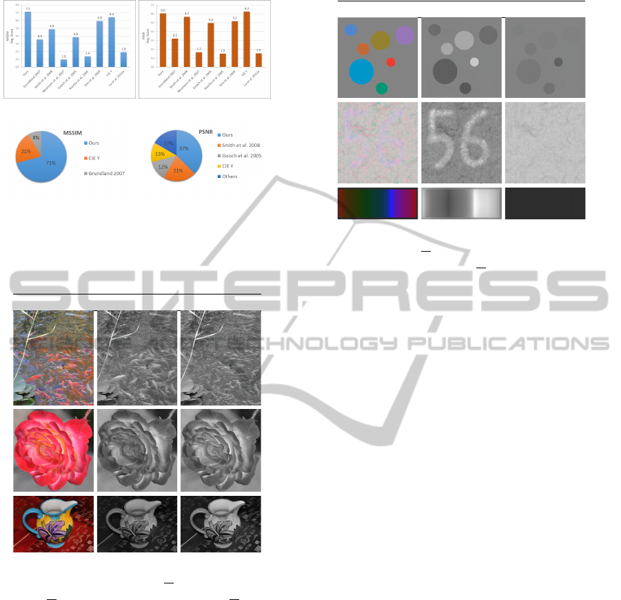
(a) (b)
(c) (d)
Figure 9: MSSIM/PSNR score statistic. (a) MSSIM aver-
age score of each method; (b) PSNR average score of each
method; (c) MSSIM No.1-hit percentage; (d) PSNR No.1-
hit percentage.
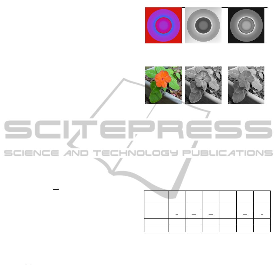
Original Our result L in CIELAB
Figure 10: Salience-preserving color-to-gray. Parameters
for each image: (1): β = 1, γ =
1
41
, α = 1, θ = 0
◦
; (2):
β = 1, γ =
1
51
, α = 1, θ = 270
◦
; (3): β = 1, γ =
1
21
, α = 0.
et al., 2009; Smith et al., 2008; Grundland and Dodg-
son, 2007; Neumann et al., 2007; Gooch et al., 2005;
Rasche et al., 2005) and CIE Y on 24 different input
images. A part of the results are shown in Fig. 8,
whose corresponding parameters are listed in Table 1.
All of the converted grayscale images are com-
pared with the original color images, and the simi-
larity is evaluated by both MSSIM and PSNR. For
each input image, the results of the 9 methods are
sorted by their MSSIM/PSNR value and scores are
given according to the ranking, i.e. the result with the
highest MSSIM/PSNR value has a score of 8, while
the lowest corresponds to 0. For each method, how
many times it wins the first place is also recorded, and
named as the ”No.1-hits”. The statistical result in Fig.
Original Our result L in CIELAB
Figure 11: Color discriminability of the algorithm. Param-
eters: (1) β = 1, γ =
1
21
, α = 1, θ = 80
◦
. (2) β = 1, γ = ∞,
α = 1, θ = 270
◦
. (3) β = 1, γ =
1
66
, α = 1, θ = 315
◦
.
9 shows that our method has the highest average score
and No.1-hits for MSSIM, and the highest No.1 hits
for PSNR. CIE Y has an advantage in average PSNR
scores because it is a linear combination of R, G and
B. Our method is competitive with it and better than
all other methods.
From the experimental results, we can see that our
method shows a satisfying salience-preserving ability.
As demonstrated in Fig. 10, many details, e.g. the
fishes in the first row, can be seen more clearly in our
results. On another aspect, grayscale distortions are
well controlled and no visible artifacts appear in the
resulting images.
Fig. 11 shows the color discriminability of our
method. Images in the middle column are our re-
sults and the right are obtained by using L channel
in the CIELAB model. Our method shows perfect
color discriminability and ordering for both discrete
color (the 1st image) and continuous color (the 2nd
and the 3rd). Especially, the 3rd image are computer-
designed isolumminance image where L = 50. The
colors cannot be distinguished in the results of L chan-
nel, while our method are able to produce grayscale
image with clear and correct color ordering.
Hence, the 4-parameter model in our method pro-
vides the ability of detail extracting and enhancing
from the color images; and optimal values for the pa-
rameters, in the sense of human vision, can be auto-
matically calculated with the MSSIM constrain. Our
method is able to preserve more details and coincide
with the human perception of color difference.
We implemented our color-to-gray conversion
method using a PES given by Press(Press et al., 1992).
As the PES has a linear time complexity (Fattal et al.,
2002), our method has a steady execution speed of
around 2 seconds per mega pixel (1024 × 1024 pixels
AutomaticColor-to-GrayConversionforDigitalImagesinGradientDomain
237

in RGB) in each optimizing iteration on a computer
with Intel Core Dou CPU 2.2GHz and 2GB memory.
The total computing time depends on the complexity
of the input image and the number of the iterations.
7 CONCLUSION
In this paper we explored the gradient domain color-
to-gray conversion. By controlling the strength of
chromatic enhancement to the luminance gradient, we
are able to obtain a salience-preserving grayscale im-
age with no visible grayscale distortion. It is based
on an observation that grayscale distortion is mainly
caused by strong chromatic differences, and Eq.(8)
aims to attenuate these strong gradient. Experiments
have proven the validity of the observation. By defin-
ing a sign function for the enhanced gradient, our
method is also able to keep correct color ordering for
isoluminance images.
Our method support automatic optimization of the
main parameters according to a structural similarity
measurement between the converted image and the
original one. This method is effective and can gen-
erate grayscale images that coincide with human vi-
sion. However, the computing efficiency of current
optimizing process is not high enough for real-time
applications. That is what we need to improve in fu-
ture works.
REFERENCES
Ancuti, C., Ancuti, C., and Bekaert, P. (2011). Enhanc-
ing by saliency-guided decolorization. In Computer
Vision and Pattern Recognition (CVPR), 2011 IEEE
Conference on, pages 257–264.
Fattal, R., Lischinski, D., and Werman, M. (2002). Gra-
dient domain high dynamic range compression. In
SIGGRAPH ’02: Proceedings of the 29th annual con-
ference on Computer graphics and interactive tech-
niques, pages 249–256, New York, NY, USA. ACM.
Gooch, A. A., Olsen, S. C., Tumblin, J., and Gooch,
B. (2005). Color2gray: Salience-preserving color
removal. In ACM SIGGRAPH 2005 Papers, SIG-
GRAPH ’05, pages 634–639, New York, NY, USA.
ACM.
Grundland, M. and Dodgson, N. A. (2007). Decolorize:
Fast, contrast enhancing, color to grayscale conver-
sion. Pattern Recogn., 40(11):2891–2896.
Ishihara, S. (1917). Test for coiour-blindness. Tokyo:
Hongo Harukicho.
Kim, Y., Jang, C., Demouth, J., and Lee, S. (2009). Ro-
bust color-to-gray via nonlinear global mapping. In
SIGGRAPH Asia ’09: ACM SIGGRAPH Asia 2009
papers, pages 1–4, New York, NY, USA. ACM.
Lu, C., Xu, L., and Jia, J. (2012a). Contrast preserving de-
colorization. In Computational Photography (ICCP),
2012 IEEE International Conference on, pages 1–7.
IEEE.
Lu, C., Xu, L., and Jia, J. (2012b). Real-time contrast
preserving decolorization. In SIGGRAPH Asia 2012
Technical Briefs, SA ’12, pages 34:1–34:4, New York,
NY, USA. ACM.
McCann, J. and Pollard, N. S. (2008). Real-time gradient-
domain painting. In SIGGRAPH ’08: ACM SIG-
GRAPH 2008 papers, pages 1–7, New York, NY,
USA. ACM.
Neumann, L.,
ˇ
Cad
´
ık, M., and Nemcsics, A. (2007). An effi-
cient perception-based adaptive color to gray transfor-
mation. In Proceedings of Computational Aesthetics
2007, pages 73– 80, Banff, Canada. Eurographics As-
sociation.
Ohta, N. and Robertson (2005). Colorimetry: Fundamen-
tals and Applications. Wiley& Sons, New York.
Pascale, D. (2003). A review of rgb color spaces ... from
xyY to R’G’B’. Babel Color.
P
´
erez, P., Gangnet, M., and Blake, A. (2003). Poisson im-
age editing. In SIGGRAPH ’03: ACM SIGGRAPH
2003 Papers, pages 313–318, New York, NY, USA.
ACM.
Press, W. H., Teukolsky, S. A., Vetterling, W. T., and Flan-
nery, B. P. (1992). Numerical Recipes in C: The Art
of Scientific Computing. Cambridge University Press,
New York, NY, USA.
Rasche, K., Geist, R., and Westall, J. (2005). Re-coloring
images for gamuts of lower dimension. Computer
Graphics Forum, 24(3):423–432.
Shevell, S. K. (2003). The Science of Color. Elsevier, Ox-
ford, UK.
Smith, K., Landes, P.-E., Thollot, J., and Myszkowski, K.
(2008). Apparent greyscale: A simple and fast conver-
sion to perceptually accurate images and video. Com-
puter Graphics Forum, 27(2):193–200.
Wang, Z., Bovik, A., Sheikh, H., and Simoncelli, E. (2004).
Image quality assessment: from error visibility to
structural similarity. Image Processing, IEEE Trans-
actions on, 13(4):600–612.
Wyszecki, G. and Stiles, W. S. (1982). Color Science: Con-
cepts and Methods, Quantitative Data and Formulae.
Wiley-Interscience, New York, NY, USA, 2 edition.
Zhou, B. and Feng, J. (2012). Gradient domain salience-
preserving color-to-gray conversion. In SIGGRAPH
Asia 2012 Technical Briefs, SA ’12, pages 8:1–8:4,
New York, NY, USA. ACM.
GRAPP2015-InternationalConferenceonComputerGraphicsTheoryandApplications
238