
Multi-Objective Capacitated Disassembly Scheduling with Lost Sales
Hajar Cherkaoui, Matthieu Godichaud and Lionel Amodeo
Institut Charles Delaunay, LOSI, Université de Technologie de Troyes, UMR 6281, CNRS, Troyes, France
Keywords: Disassembly Scheduling, Remanufacturing, Multi-Objective, Optimization, Lost Sales, Nsga-II.
Abstract: Disassembly scheduling is one of the important problems in reverse logistic decisions. This paper focuses
on this problem with capacity restrictions on disassembly resources, lost sales, multiple products and
without part commonality. A model with two objectives is developed and optimized by a multi-objective
approach. The first objective is a sum of several costs to minimize: setup cost, inventory cost, and over
capacity penalty cost. The second objective is a measure of the service level. Considering the complexity of
this model, a genetic algorithm is developed (NSGA-II) to obtain a set of Pareto-optimal solutions, the
results are compared with those calculated by a mixed integer programming model. Results of
computational experiments on randomly generated test instances indicates that the genetic algorithm gives
good quality solutions up to all problem sizes in a reasonable amount of computation time whereas linear
programming solvers do not give solution in reasonable time.
1 INTRODUCTION
Nowadays, due to environmental and economic
reasons, more and more companies acknowledge that
reverse logistic is a part of the supply chain as
important as production or distribution. Disassembly
process consists in separating recovered products to
generate components which can be reused or be
conditioned safely for the environnement.
Disassembly scheduling defines how many products
to disassemble given the demands for components in
each period of a finite horizon planning. In this paper
we consider two-level product structure disassembly
scheduling problem with setup times, lost sales,
multi-products types and limited capacity. Part
commonality between products is not considered in
this paper.
The goal of this study is to develop a
optimization tool for this problem with two objective:
total cost and service level. To our knowledge, the
disassembly scheduling problem with lost sales has
not been studying in literature. Lost sales allow
selecting demand to be satisfied and minimizing
inventory surplus that is inherent to disassembly
scheduling problem. In the following section, we
start by a literature review of disassembling
problems. In section 3, a mathematical formulation of
the problem is introduced. In section 4, a meta-
heuristic based on genetic algorithm NSGA-II is
developped for large instance when CPLEX solver
do not give solutions in reasonable time. Finally,
section 5 explores the performances of the meta-
heuristic and compares results with solutions given
by solving the mixed integer programming model.
Concluding remarks and future research goals will be
given in section 6.
2 LITERATURE REVIEW
In this section we present various problems in
disassembly system studied in literature. Gupta and
Taleb (1994) defined and characterized the basic
disassembly scheduling problem for a single product
type, without explicit objective function and
suggested an algorithm that is a reversed Material
Requirement Planning (MRP). This problem was
further extended to include commonality parts by
Guta and Taleb (1997) for multiple product case.
Disassembly scheduling can be classified into
deterministic and non-deterministic problems which
incorporate random factors in the models, Inderfurth
and Langella (2006) developed two heuristics which
take into consideration stochastic disassembly
yields, with multiple product types, parts
commonality, two-level product structure. Here we
interested on deterministic problems. When set up
costs is considered in the objective function, lost
sizing decision have to be made. We note that
methodologies for lot sizing in production and
172
Cherkaoui H., Godichaud M. and Amodeo L..
Multi-Objective Capacitated Disassembly Scheduling with Lost Sales.
DOI: 10.5220/0005231901720178
In Proceedings of the International Conference on Operations Research and Enterprise Systems (ICORES-2015), pages 172-178
ISBN: 978-989-758-075-8
Copyright
c
2015 SCITEPRESS (Science and Technology Publications, Lda.)

assembly scheduling cannot be applied to
disassembly due to their divergence characteristic,
see Kim et al. (2007) for more details of the
divergence characteristic. Resource capacity
restriction also complicate the problem. Lee et al.
(2002) considered the capacitated problem, and
proposed an integer programming model for the case
of single product type. Lee and Xirouchakis (2004)
and Kim et al. (2003) proposed integer programming
models to determine the disassembly scheduling of
used products in order to satisfy the demand of their
parts over a planning horizon, considering various
situations involving costs and capacity. Kim et al.
(2006) developed a two-phase heuristic to minimize
of set up, disassembly operation and inventory-
holding costs. Lee et al. (2006) developed an integer
programming model considering capacity restriction,
a two stage solution approach is proposed. Barba et
al (2008) present an algorithm for reverse MRP with
various lot sizing heuristics. Kim et al. (2010)
consider the problem that minimizes the total cost
that is sum of setup cost and inventory holding cost,
they suggested a branch and bound algorithm that
incorporates Lagrangian relaxation technique to
obtain good lower and upper bounds. In this study
we test the model with their instances. Kim and Lee
(2011) proposed a heuristic for multi-period
disassembly leveling and scheduling. To out
knowledge, there is no study on disassembly lot
sizing with lost sales.
There are several references on production lot
sizing with lost sales. Xiao Liu and Freng Chu
(2004) address the capacitated lot sizing problem
with lost sales, they developed a dynamic
programming algorithm to solve the problem. Absi
et al (2013) deals with the same problem, they
proposed a non-myopic heuristic based on a probing
strategy and refining procedure. Their approaches
can not be applied in disassembly. Indeed, there is
one supply product source for several component
demands and hence when a component demand is
satisfied and may be cause stockout or inventory
surplus for others components.
Various objectives can be considered in lot
sizing problems. Jafar and Mansoor (2011)
addressed the lot-sizing problem with supplier
selection, they developed two multi-objective mixed
integer non-linear models for multi-period lot-sizing
problems with multiple products and multiple
suppliers, three objectives are considered cost,
quality and service level. Ayyuce et al. (2013) deals
with multi-objective optimization of a stochastic
disassembly line balancing problem, they proposed a
genetic algorithm which generates Pareto-optimal
solutions considering two different fitness evaluation
approaches.
To the best of the authors’ knowledge, no one
has addressed the optimization of capacitated
disassembly scheduling with lost sales and multi-
objective approach. In this paper we compare an
exact method for mono-objective and a meta-
heuristic for multi-objective.
3 MODEL FORMULATION
In this section we present the mixed integer
programming model of the problem. Before
formulating the mathematical model, the
disassembly process is described first.
A parent (root) item can be disassembled to
produce a specific number of child (leaf) items.
Given a set of root items, the demand of each leaf
items of all roots is given over a time horizon. Each
period has a normal production capacity, exceeding
this capacity will result a penalty cost. If the demand
of a leaf item is not met in a period it will be
considered as lost sales. The problem is to determine
the quantity and timing of disassembling all root
items to satisfying demand of their leaf items over
the planning horizon subject to capacity restrictions
in each period, respecting a particular service level.
In this paper we consider two objectives: total
cost and service level. The first objective is to
minimize the sum of purchase, inventory holding,
and disassembly costs. The second one is to
maximize the service level. The cost of not satisfied
demand is difficult to assess and we cannot combine
cost and quantity in the same objective function, thus
we consider in this model one objective (Total cost)
and we include the second (Service level) as a
constraint.
A. Model parameters and decision variables
The notations used are summarized below.
Indices:
r Index for root items, r=1,2,…, R
i Index for leaf items, i=1,2,…,N
t Index for periods, t=1,2,…,T
Parameters
Setup cost of parent item r.
Capacity available, in time, in period t.
Parent of leaf item i.
Disassembly operation time of root item r.
Inventory holding cost of item i.
Penalty cost disassembly time in period t.
Demand of item i in period t.
Multi-ObjectiveCapacitatedDisassemblySchedulingwithLostSales
173

Number of unit of items i obtained by
disassembly of one unit of its parent item r.
Initial inventory of item i.
Large Number.
Maximal lost sales level (%).
Decision variables
= 1 if there is a setup for root item r in period
t, 0 otherwise.
Disassembly quantity of root item r through
period t.
Disassembly over-time in period t.
Inventory level of leaf item i at the end of
period t.
Lost sales for each leaf item I in period t.
B. Model assumptions
Assumptions made in this model are summarized as
follows:
(a) Demands for leaf items are given and
deterministic;
(b) Lost sales is allowed, hence demand can be not
satisfied;
(c) The disassembly process is perfect, all parts are in
perfect quality, no defective are considered;
(d) Disassembly operation times are given and
deterministic;
C. Mathematical formulation
In this study we solve the problem using two
approaches.
The first case is a mixed integer program (MIP)
where the first objective is the objective function
and the second objective is a constraint. The
constraint level is varying it to obtain different
solutions for the same instance.
We note that in this model we consider the total lost
sales level which can be calculated as:
TotalLostSalesLevel L
/
d
and then total service level can be deducted :
1
With above parameters and decision variables, the
MIP is given bellow.
∑∑
∗
∑∑
∗
∑
∗
(1)
Subject to
,
,
∗
forall
t2,…Tandi1,…N
(2)
∗
forallt1,…Tandr1,…
R
(3)
∑
g
∗
C
for all t=1,…T
(4)
for all t=1,…T and i=1,…N
(5)
∑∑
L
/
∑∑
d
(6)
,
0
(7)
Objective function (1) is the Total cost which is the
sum of setup cost, expected inventory holding and
penalty costs, production costs are not considered in
this study.
The constraint are the following :
‐ (2) define the inventory flow conservation of
leaf items at the end of each period (
,
) is an
input data.
‐ (4) Ensure that a setup is performed in a period
when disassembly operation is performed.
‐ (5) Enforces the capacity feasibility.
‐ (7) State the upper bound available of lost sales
level; we note that maximizing the total service
level equivalent minimizing the total lost sales
level.
‐ (8) Defines the domain of variables.
The second case we solve the problem by using the
NSGA-II algorithm that considers multiple
objectives:
∑∑
∗
∑∑
∗
∑
∗
∑∑
Subject to : Constraints (1) to (6) and (8).
4 MULTI-OBJECTIVE GENETIC
ALGORITHM
Generally, based on a population search Multi-
Objective Evolutionary Algorithm (MOEA) can
present a set of non-dominated or Pareto optimal
solutions. In this study we consider two objectives,
total cost and service level. To solve the model in this
paper we use Non-dominated Sorting Genetic
Algorithm II (NSGA-II), one of the MOEAs
frequently used in many optimization problems as
the best technique to generate Pareto frontiers, which
has been proposed by Deb et al. (2000). Moreover,
the NSGA-II has been consistently uses in several
research articles which deals with supply chain
problems see Godichaud et al., D. Sanchez et al. and
Li et al.
D. NSGA-II Principle
This algorithm uses a fixed-sized population. We
start by initializing the population then the population
is sorted based on non-domination criteria into
several fronts. The first front is a completely non-
dominated set in the current population and the
ICORES2015-InternationalConferenceonOperationsResearchandEnterpriseSystems
174

second front being dominated by the individuals in
the first front only and so on. Each individual in each
front is assigned fitness value. We said that solution
is dominated by solution if only is better than
with regard to all objectives, or is better than
with regard to other objectives. This process is
continues until all fronts are identified. In addition to
fitness value we calculate the crowding distance
which is a measure of how close an individual is to
its neighbors, we used it in order to maintain
diversity in the population.
E. NSGA-II algorithm
, of size n;
Create child population
using binary tournament
selection, recombination and mutation;
While (stopping criterion)
We create a new population
which
combine
(parent) and
(child)
Sort
by non-domination
Assign a fitness equal to its non-domination level
for each solution, identify levels
,1,2,…
Computed the crowding distance of each solution
Set new population
Set i=1
While
|
|
|
|
do
Add
to
Set i=i+1
end while
Set
|
|
If 0
Sort solutions by descending crowding
distance
1
Add
of
to
end for
end if
end while
F. Encoding
In this study, the decisions variables are
,
,
,
and
, among which
is a binary variable (0-1), and
the others are positive variables of integer numbers.
Generally, in literature, setup variables are used to
encode solutions and integer variables are deduced
based of the properties of the model. These properties
are not sufficient for the problem with with lost sales
and integer varaibles can not be computed from
,
and thus, we encode
as chromosomes.
G. Initial population
In this study, population of candidate solution
is
randomly generated according to an uniform
distribution. We use a random integer generator for
with respect to the bounding conditions.
H. Selection and Evaluation
Capacity constrains and objective functions are used
to evaluate the objectives of each chromosome, we
note that there are two objective function values for
each one. We use the constrained tournament
method because of its ability to satisfy constraints
and at the same time perform selection based on
fitness.
This operator involves running several tournaments
among a few individuals chosen at random from the
population and the one with best fitness (winner) is
selected for crossover.
I. Crossover and Mutation
One crossover point is used. Genes from beginning
of chromosome to the crossover point is copied from
one parent, and the rest is copied from the second
parent, at the end we obtained two children. After
this we mutate on chromosome by changing one
more variable in some way by random. Crossover
and mutation are performed with a given probability.
Values are mentioned in the next section.
5 COMPUTATION
EXPERIMENTS
The NSGA-II algorithm tested in this paper was
coded in Java and run on a personal computer with a
five processors operating at 2.60 GHz clock speed.
J. Test instances
For the test, instances are generated as in (H.-J.
Kim and P. Xirouchakis, 2010). U(a,b) is the discrete
uniform distribution with a range of [a,b].
We generated 10 instances for each number of
root items (10,20,30), three number of
children generated from a discrete uniform
distribution with a rang U(1,10), U(10,100),
and U(100,1000) for low, medium, and large
respectively ,and three number of periods
(10,20,30);
∶Setup cost for each root was generated
from U(1000,5000);
∶ For each root the number of child were
generated from U(1,5);
∶Demand was generated from U(50,200);
∶ Inventory holding costs were generated
from U(1,10);
∶ Penalty costs for overtime were
generated from U(5,15);
Multi-ObjectiveCapacitatedDisassemblySchedulingwithLostSales
175
∶Disassembly time was generated from
U(1,3);
∶Initial inventory was generated from
(20,100).
∶ Available aggregate capacity in each
period is set to 540,480 and 400 with
probabilities, 0.3,0.5,0.2
K. Parameters setting
Different tests with different parameters were made
to choose the efficient parameters for the algorithm.
The following control parameters for genetic
algorithm are the ones we used in our case study:
Maximum generation 1500.
Population size 100.
Mutation probabilityCoef
0,2.
Crossover probabilityCoef
0,9.
L. Computational Results
In this section, we apply the GA discussed earlier to
solve the model proposed and to show the
effectiveness of our GA meta-heuristic firstly we
compare the NSGA-II performances with those of
Cplex 12.5 software, in terms of computation time
and solution quality to solve the small-sized problem
and after we present the strength of the NSGA-II to
solve all sizes instances.
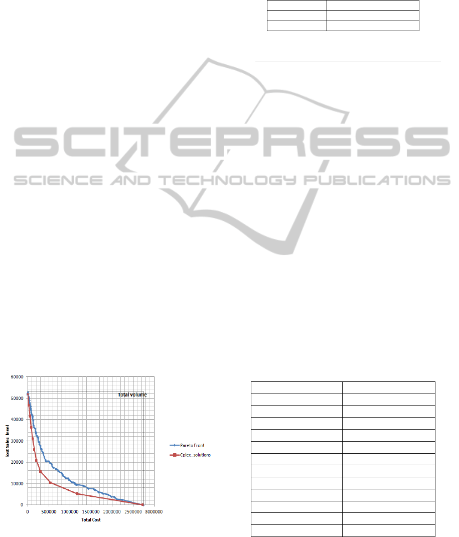
The figure 1 present Pareto front obtained with
NSGA-II for the first instance (10 periods, 10 roots,
low number of children), the Pareto contains 100
solutions. We present also 11 exact algorithm
solutions solved with mono-objective for 11
different percentages of lost sales level. We note that
each solution obtained is a point of the optimal
Pareto front.
To show the quality of our results we will
compare the two fronts: the first obtained by Cplex
(optimal pareto solution) and the second obtained by
NSGA-II.
Figure 1: Example of Pareto front obtained with GA (100
solutions) and some exact algortihm solutons (11
solutions).
To compare our curves we use the Hyper Volume
indicator. Readers wishing more detailed description
of the algorithm can be referred to Deb.
Table 1 present the hyper volume values:
Table 1: Hyper volume values for Cplex and NSGA-II.
Hyper Volume
Cplex 0.829
NSGA-II 0.826
0.36%
The gap indicates that the front solutions of NSGA-
II is 99,64% close to the optimal front obtained by
Cplex. Moreover the decision maker has several
choices in terms of solutions (100 by NSGA-II
against 11 by Cplex).
Here, the heuristic solutions are compared with
Cplex solutions to assess the benefits of increasing
the CPU time limit. Concerning the exact method
(case 1), we solve the problem on mono-objective.
This table summarizes the computation time of one
instance with 10 periods, 10 roots and low number
of children. As mentioned in mathematical model
there is a constraint of lost sales level: LMax, in this
experiment we change the LMax value and we
evaluate the objective function. In this test we used
Cplex software to obtain solutions.
For this instance for each lost sales level value
we allowed Cplex to run for maximum 3000sec to
avoid excessive computation times and we fixed the
absolute tolerance on the gap between the best
integer objective and the objective of the best node
remaining at 0.01.
Table 2: CPU time for different lost Sales level.
Lost Sales level (%) Objective CPU(sec)
0 1.71
10 5.89
20 49.30
30 1138.43
40 1804.52
50 466.61
60 98.88
70 59.77
80 21.39
90 6.19
100 0
Total time
3652,69
We reported CPU time in second for the instance
ICORES2015-InternationalConferenceonOperationsResearchandEnterpriseSystems
176

example in table 2, the total time to compute
solutions for each percentage of lost sales level (11
solutions) is:
3652,69
On the other side the total time to obtain the
Pareto front which provides 100 solutions with the
NSGA-II algorithm (considering mathematical
model case 2) for the same instance is:
Total
4sec (see the table 2 in the next
section). We kept a large number of solution to
analyse the behaviour of the algorithm. In practice,
decision makers have to choose only one solution
based on its preferences. Multi criteria decision
making can be used to this end with the NSGA-II
solutions as an input.
Total
≪Total
(4sec<<3652,69sec)
Table 3: CPU time in seconds of Kim problem instances.
Number of
root items
Number of
children
Number of
periods
CPU(sec)
10
20
30
Low
Medium
Large
Low
Medium
Large
Low
Medium
Large
10
20
30
10
20
30
10
20
30
10
20
30
10
20
30
10
20
30
10
20
30
10
20
30
10
20
30
4
7
10
19
37
66
299
414
741
7
11
15
47
86
115
618
776
1271
11
20
26
80
121
171
973
2278
3317
Genetic algorithm is much faster than Cplex,
without taking into consideration the number of
solution found. Genetic algorithm gives solutions
that are very close to optimal ones within very short
computational time. Hence the efficiency of the
genetic algorithm provides the decision maker a
huge choice in terms of solution quality and in short
time. Before presenting results we note that from 30
periods with medium number of children Cplex
could not give solutions. In this section the table 3
summarize the computation time of the GA for all
instances.
We observe that the computation time increases
quickly as the number of the periods, on the other
side it does not increase apparently as the numbers of
root items increase.
6 CONCLUSIONS
In this paper, we addressed the multi-products
capacitated disassembly scheduling with setup times
and lost sales. To our knowledge, it the first time that
disassembly scheduling problem with lost sales is
investigated. We formulated a multi-objective
optimization model, and propose a genetic algorithm
NSGA-II for solving the problem. The objectives
considered are (1) Minimizing the total cost and (2)
Maximizing the service level. The performance of
NSGA-II is investigated by comparing its results
with those obtained by exact method on mono-
objective sample (270 test problems) randomly
generated (Kim et al.-2009- instances). This
comparison shows that the NSGA-II give solution
with good quality in reasonable time while Cplex
software does not. This research can be extended in
several ways. New mathematical formulation
approaches can be developed considering multi level
product structure and parts commonality constraints.
Uncertainties such as stochastic demands or
stochastic disassembly times have to be considered.
The method can also be improved by using other
dominance criterion to reduce the number of solution
and be developing hybridization. Properties of the
model should also be investigated to improve
encoding of solutions.
REFERENCES
S. M. Gupta and K. N. Taleb, “Scheduling disassembly,”
International Journal of Production Research, vol. 32,
no. 8, pp. 1857–1866, 1994.
Multi-ObjectiveCapacitatedDisassemblySchedulingwithLostSales
177

H.-J. Kim, D.-H. Lee, and P. Xirouchakis, “Disassembly
scheduling: literature review and future research
directions,” International Journal of Production
Research, vol. 45, no. 18–19, pp. 4465–4484, 2007.
K. N. Taleb and S. M. Gupta, “Disassembly of multiple
product structures,” Computers & Industrial
Engineering, vol. 32, no. 4, pp. 949–961, Sep. 1997.
K. Inderfurth and I. M. Langella, “Heuristics for solving
disassemble-to-order problems with stochastic yields,”
OR Spectrum, vol. 28, no. 1, pp. 73–99, Jan. 2006.
D.-H. Lee, P. Xirouchakis, and R. Zust, “Disassembly
Scheduling with Capacity Constraints,” CIRP Annals -
Manufacturing Technology, vol. 51, no. 1, pp. 387–
390, 2002.
D.-H. Lee and P. Xirouchakis, “A two-stage heuristic for
disassembly scheduling with assembly product
structure,” J Oper Res Soc, vol. 55, no. 3, pp. 287–
297, 2004.
H.-J. Kim, D.-H. Lee, P. Xirouchakis, and R. Züst,
“Disassembly Scheduling with Multiple Product
Types,” CIRP Annals - Manufacturing Technology,
vol. 52, no. 1, pp. 403–406, 2003.
H.-J. Kim, D.-H. Lee, and P. Xirouchakis, “Two-phase
heuristic for disassembly scheduling with multiple
product types and parts commonality,” International
Journal of Production Research, vol. 44, no. 1, pp.
195–212, 2006.
H.-J. Kim, D.-H. Lee, and P. Xirouchakis, “Two-phase
heuristic for disassembly scheduling with multiple
product types and parts commonality,” International
Journal of Production Research, vol. 44, no. 1, pp.
195–212, 2006.
Y. Barba-Gutiérrez, B. Adenso-Díaz, and S. M. Gupta,
“Lot sizing in reverse MRP for scheduling
disassembly,” International Journal of Production
Economics, vol. 111, no. 2, pp. 741–751, Feb. 2008.
H.-J. Kim and P. Xirouchakis, “Capacitated disassembly
scheduling with random demand,” International
Journal of Production Research, vol. 48, no. 23, pp.
7177–7194, 2010.
B. Adenso-Diaz, S. Carbajal, and S. Lozano,
“Disassembly scheduling of complex products using
parallel heuristic approaches,” in 2010 IEEE/ACS
International Conference on Computer Systems and
Applications (AICCSA), 2010, pp. 1–4.
X. Liu, C. Wang, F. Chu, and C. Chu, “A forward
algorithm for capacitated lot sizing problem with lost
sales,” in Fifth World Congress on Intelligent Control
and Automation, 2004. WCICA 2004, 2004, vol. 4,
pp. 3192–3196 Vol.4.
N. Absi, B. Detienne, and S. Dauzère-Pérès, “Heuristics
for the multi-item capacitated lot-sizing problem with
lost sales,” Computers & Operations Research, vol.
40, no. 1, pp. 264–272, Jan. 2013.
J. Rezaei and M. Davoodi, “Multi-objective models for
lot-sizing with supplier selection,” International
Journal of Production Economics, vol. 130, no. 1, pp.
77–86, Mar. 2011.
D.-H. Kim and D.-H. Lee, “A heuristic for multi-period
disassembly leveling and scheduling,” in 2011
IEEE/SICE International Symposium on System
Integration (SII), 2011, pp. 762–767.
A. Aydemir-Karadag and O. Turkbey, “Multi-objective
optimization of stochastic disassembly line balancing
with station paralleling,” Computers & Industrial
Engineering, vol. 65, no. 3, pp. 413–425, Jul. 2013.
M. Schoenauer, K. Deb, G. Rudolph, X. Yao, E. Lutton, J.
J. Merelo, and H.-P. Schwefel, Eds., Parallel Problem
Solving from Nature PPSN VI, vol. 1917. Berlin,
Heidelberg: Springer Berlin Heidelberg, 2000.
M. Godichaud, Amodeo L., Multi-objective Optimization
of Supply Chains with Returns, International
Conference on Metaheuristics and Nature Inspired
Computing, META 2012, Sousse, Tunisia, 27-31
October 2012.
D. Sánchez, L. Amodeo, and C. Prins, “Meta-heuristic
Approaches for Multi-objective Simulation-based
Optimization in Supply Chain Inventory
Management,” in Artificial Intelligence Techniques
for Networked Manufacturing Enterprises
Management, L. Benyoucef and B. Grabot, Eds.
Springer London, 2010, pp. 249–269.
Li X., Yalaoui F., Amodeo L., Chehade H., Metaheuristics
and exact methods to solve a multiobjective parallel
machines scheduling problem, Special Issue on
Advanced Metaheuristics For Integrated Supply Chain
Management, Journal of Intelligent Manufacturing
(ISI), Vol 23, pp 1179-194, 2012.
ICORES2015-InternationalConferenceonOperationsResearchandEnterpriseSystems
178
