Re-aggregation Approach to Large Location Problems

Matej Cebecauer and

Lubo

s Buzna

University of Zilina, Univerzitna 8215/1, SK-01026 Zilina, Slovakia

Keywords:

Location Problem, Heuristics, Aggregation, OpenStreetMap.

Abstract:

The majority of location problems are known to be NP-hard. An aggregation is a valuable tool that allows to

adjust the size of the problem and thus to transform it to the problem that is computable in a reasonable time.

An inevitible consequence is the loss of the optimality due to aggregation error. The size of the aggregation

error might be signiﬁcant, when solving spatially large problems with huge number of customers. Typically,

an aggregation method is used only once, in the initial phase of the solving process. Here, we propose new

re-aggregation approach. First, our method aggregates the original problem to the size that can be solved by

the used optimization algorithm, and in an each iteration the aggregated problem is adapted to achieve more

precise location of facilities for the original problem. We use simple heuristics to minimize the sources of

aggregation errors, know in the literature as, sources A, B, C and D. To investigate the optimality error, we use

the problems that can be computed exactly. To test the efﬁciency of the proposed method, we compute large

location problems reaching 80000 customers.

1 INTRODUCTION

The location problem consists of ﬁnding a suitable set

of facility locations from where services could be efﬁ-

ciently distributed to customers (Eiselt and Marianov,

2011; Daskin. M., 1995; Drezner, 1995). Many lo-

cation problems are known to be NP-hard. Conse-

quently, the ability of algorithms to compute the op-

timal solution quickly decreases as the problem size

is growing. There are two basic approaches how to

deal with this difﬁculty. First approach is to use a

heuristic method, which, however, does not guaran-

tee that we ﬁnd the optimal solution. Second ap-

proach is to use the aggregation, that lowers the num-

ber of customers and candidate locations. The aggre-

gated location problem (ALP) can be solved by ex-

act methods or by heuristics. Nevertheless, aggrega-

tion induces various types of errors. There is a strong

stream of literature studying aggregation methods and

corresponding errors (Francis et al., 2009; Erkut and

Bozkaya, 1999). Various sources of aggregation er-

rors and approaches to minimize them are discussed

by (Hillsman and Rhoda, 1978; Current and Schilling,

1987; Erkut and Bozkaya, 1999).

Here, we are speciﬁcally interested in ﬁnding the

efﬁcient design of a public service system that is serv-

ing spatially large geographical area with many cus-

tomers. Customer are modeled by a set of demand

points (DP) representing their spatial locations (Fran-

cis et al., 2009). To include all possible locations of

customers as DPs is often impossible and also unnec-

essary. In similar situations the aggregation is valu-

able tool to obtain ALP of computable size.

The basic data requirements for public service

system design problem are location of DPs and the

road infrastructure that is used to distribute services

or access the service centers. In this paper we use vol-

unteered geographical information (VGI) to extract

road infrastructure and locations of customers. VGI

is created by volunteers, who produce data through

Web 2.0 applications and combine it with the pub-

licly available data (Goodchild, 2007). We use data

extracted from the OpenStreetMap (OSM), that is one

of the most successful examples of VGI. For instance,

in Germany the OSM data are becoming comparable

in the quality to commercial providers (Neis et al.,

2011). Road and street networks in the UK reaches

good precision as well (Haklay, 2010). Therefore,

OSM is becoming an interesting and freely available

alternative to commercial datasets.

We combine the OpenStreetMap data with avail-

able residential population grid (Batista e Silva et al.,

2013) to estimate the demand that is associated to

DPs.

It is well known, that the solution that is pro-

vided by a heuristic method using more detailed data

Cebecauer M. and Buzna L..

Re-aggregation Approach to Large Location Problems.

DOI: 10.5220/0005222300420050

In Proceedings of the International Conference on Operations Research and Enterprise Systems (ICORES-2015), pages 42-50

ISBN: 978-989-758-075-8

 2015 SCITEPRESS (Science and Technology Publications, Lda.)

Figure 1: Schematic illustrating the generation of DPs.

is often better than a solution achieved by the exact

method, when solving aggregated problem (Hodgson

and Hewko, 2003; Andersson et al., 1998). Often, ag-

gregation is used only in the initial phase of the solv-

ing process, to match the problem size with the perfor-

mance of the used solving method. In this paper, we

propose a re-aggregation heuristic, where the solved

problem is in each iteration modiﬁed to minimize the

aggregation error in the following iterations. Our re-

sults show that the re-aggregation may provide bet-

ter solutions than solution obtained by exact methods

when using aggregated data or solutions found by the

heuristic method which uses aggregation only once.

The paper is organized as follows: section 2 in-

troduces the data processing procedure. The re-

aggregation heuristic is explained in section 3. In sec-

tion 4, we brieﬂy summarize the p-median problem,

that we selected as a test case. Results of numerical

experiments are reported in section 5. We conclude in

section 6.

2 DATA MODEL

The OSM provides all necessary data to generate DP

locations and to extract the road network. To esti-

mate the position of demand points we use OSM lay-

ers describing positions of buildings, roads, residen-

tial, industrial and commercial areas. To generate DPs

we use a simple procedure. First, we generate spa-

tial grid, which consists of uniform square cells with

a size of 100 meters. For each cell we extract from

OSM layers elements that are situated inside the cell.

Second, DPs are located as centroids of cells with a

non empty content. The process of generating DPs

is visualized in Figure 1. Third, generated DPs are

connected to the road network and we compute short-

est paths distances between them. Finally, we calcu-

late Voronoi diagrams, while using DP as generating

points, and we associate with each DP a demand by

intersecting Voronoi polygons with residential popu-

lation grids produced by (Batista e Silva et al., 2013).

3 RE-AGGREGATION

HEURISTIC

In this section we describe our re-aggregation ap-

proach. The main goal is to re-aggregate solved prob-

lem in each iteration to achieve more precise locations

of facility in the following iterations. Aggregation is

an essential part of the heuristic and it leads to loca-

tions errors (Francis et al., 2009; Erkut and Bozkaya,

1999). To minimize the effect of aggregation errors

we need to understand the possible sources of errors.

Therefore, we start by a brief summary of known

sources of aggregation errors that are related to the

input data. These sources of errors are in the litera-

ture denoted as A, B, C and D. We describe meth-

ods how to reduce them (Current and Schilling, 1987;

Hodgson and Neuman, 1993; Hodgson et al., 1997;

Erkut and Bozkaya, 1999). To supplement this dis-

cussion we also point at the sources of errors that are

often made by designers of public systems (Erkut and

Bozkaya, 1999).

3.1 Aggregation Errors

Aggregation errors are caused by the loss of informa-

tion, when DP are replaced by aggregated demand

points (ADP). (Hillsman and Rhoda, 1978) named

these errors as source errors and introduced source A,

B and C errors. Elimination of source A and B errors

was studied by (Current and Schilling, 1987). Mini-

mization of the source C error was analysed in (Hodg-

son and Neuman, 1993). Source D error and possibil-

ities how it can be minimized were studied in (Hodg-

son et al., 1997). We summarize source error in Table

Some errors are also often made by designers or

decision makers, who are preparing the input data or

evaluating the aggregation errors. Examples of such

errors can be use of uniform demand distribution, ag-

gregation method that is ignoring population clusters,

or incorrect methods used to measure the aggregation

error (Erkut and Bozkaya, 1999).

The algorithm we are proposing is minimizing all

source errors A, B, C and D. To aggregate DPs we use

row-column aggregation method proposed by (Ander-

sson et al., 1998), which considers population clus-

ters. To evaluate the aggregation error in numerical

experiments, we measure optimality error, which is

commonly use metrics in the location analysis (Fran-

cis et al., 2009; Erkut and Bozkaya, 1999).

Re-aggregationApproachtoLargeLocationProblems

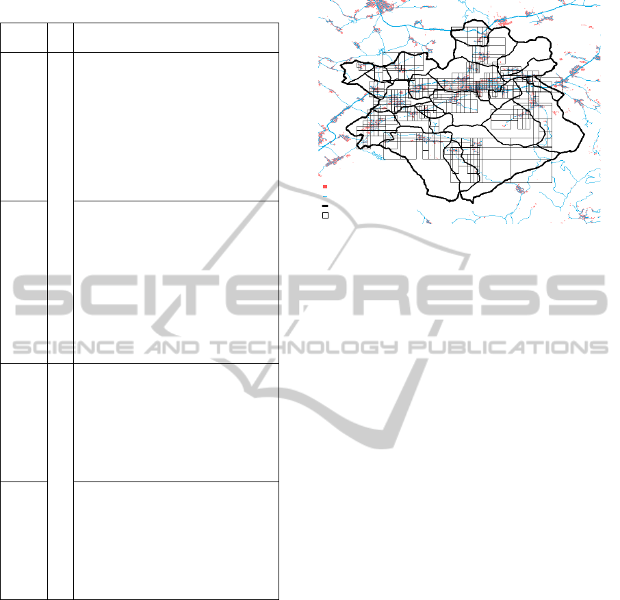
Table 1: Types of source errors.

Error

Description

type

source A error

eliminated by preprocessing the input data

This error is a result of wrongly

estimated distance between ADPs

a and b, when measuring the dista-

nce only between corresponding

centroids.

Elimination

Replace the distance by the sum

of distances from all DPs agg-

regated in the ADP a to the

centroid of ADP b.

source B error

It is a speciﬁc case of source A error.

If ADP a is a candidate location for

a facility, and at the same time it re-

presents a customer, the distance be-

tween facility location a and custo-

mer a is incorrectly set to zero value.

Elimination

Replace the zero distance

by the sum of all distances

from DPs aggregated in the ADP a

to the centroid of the ADP a.

source C error

eliminated by postprocessing the results

All DPs aggregated in the same

ADP are assigned to the same

facility.

Elimination

Re-aggregate ADPs and ﬁnd the

closest facility for all DPs.

source D error

It is consequence of establishing

facilities in ADPs and not in DPs.

Elimination

Find the facility location by

disaggregating ADPs in the close

neighborhood of located facilities.

3.2 Aggregation Method

To aggregate DP, we use row-column aggregation

method proposed by (Francis et al., 1996; Andersson

et al., 1998). In this part we introduce original row-

column aggregation method and our adaptation to the

spatially large geographical areas with many munici-

palities.

First, we introduce three basics steps of the

original aggregation method (Francis et al., 1996;

Andersson et al., 1998):

STEP 1: Generate irregular grid for the whole

geographical area of the problem.

STEP 2: Select a centroid (ADP) of each grid cells.

STEP 3: Assign DP to the closest ADP.

building

road

municipalities boundary

cell of the aggregation method grid

Figure 2: Map of the area after application of the row-

column aggregation method to each administrative zone

separately. The aggregation procedure results in 1000

ADPs.

The irregular grid, with c columns and r rows,

is obtained by solving the c-median problem on the

projection of the DPs to the x-axis, and the r-median

problem on the projection of the DPs to the y-axis.

The border lines deﬁning the rows and columns are

positioned in the middle between facilities that has

been found by solving the one dimensional location

problems (Francis et al., 1996). Next in the step 2, for

each call of the grid, we extract the subnetwork of the

road network that intersects with the area of the cell.

ADP is found by solving the 1-median problem for

each individual subnetwork (Andersson et al., 1998).

Finally, each DP is assigned to the closest ADP.

We slightly modiﬁed this approach by applying

it to each individual administrative zone separately.

This allows to approximate population clusters more

precisely and thus it helps to minimize the aggrega-

tion error. In the Figure 2 is visualised the result of

the aggregation obtained by the row-column aggrega-

tion method.

3.3 Re-aggregation Algorithm

The proposed heuristic algorithm consists of several

phases. Main parameters of the algorithm are de-

scribed in Table 2. Re-aggregation algorithm is com-

posed from phases that are executed in the following

order:

Phase 0: Initialization

Set i = 0 and prepare ALP aggregating the input data.

The results be s ADPs and the corresponding distance

matrix.

Phase 1: Elimination of Source A and B Errors

ICORES2015-InternationalConferenceonOperationsResearchandEnterpriseSystems

Table 2: Parameters of the re-aggregation algorithm.

Symbol Description

s Initial number of ADPs.

m Maximal number of ADPs.

r Maximal number of iterations.

Radius of ADP neighbourhood. This

parameter divides the set C of all

ADPs into two subsets A, B ⊂ C, where

A ∩ B =

0 and A ∪ B = C. Subset A

includes all ADPs that

are are located from the closest facility at

distance less than ε. Subset B is

deﬁned as B = C − A.

Percentage of ADPs

that are re-aggregated in each iteration.

p-LA

Algorithm for solving p-location

problem.

1-LA

Algorithm for solving 1-location

problem.

Update the distance matrix accounting for source A

and B errors.

Phase 2: Location of Facilities

Solve ALP using p-LA algorithm. As a result we ob-

tain located facilities.

Phase 3: Elimination of Source C and D Errors

To minimize the source C error reallocate DPs to the

closest facilities.

To minimize the source D error decompose the prob-

lem into p location problems each consisting of one

facility location and of all associated DPs. Each de-

composed problem is solved using 1-LA algorithm.

As a result we obtain p new locations of facilities.

Phase 4: Re-aggregation

If all ADPs with an established facility are constituted

by only one DP or if i > r then terminate. Otherwise,

considering the parameter ε, divide the set of DPs into

two subsets A and B. Move from subset B into the

subset A all ADPs that include at least one DP that

has shorter distance to another facility than its ADP

centroid. De-aggregate each ADP in the subset A to

λ new ADPs using aggregation method from initial

phase 0 and update the value of parameter s. While

s > m than randomly select one ADP from subset B

and aggregate it with the closest ADP from the subset

B. Increment i by 1 and go to the phase 1.

4 THE P-MEDIAN LOCATION

PROBLEM

The number of existing location problems is over-

whelming (Eiselt and Marianov, 2011; Daskin. M.,

1995; Drezner, 1995). To evaluate the optimality

error and the time efﬁciency of the proposed re-

aggregation algorithm, we use the p-median problem,

which is one of the most frequently studied and used

location problems (Hakimi, 1965; Calvo and Marks,

1973; Berlin G N et al., 1976; Jan

cek et al., 2012).

This problem includes all basic decisions involved in

the service system design. The goal is to locate ex-

actly p facilities in a way that the sum of weighted

distances from all customers to their closest facilities

is minimized. The problem is NP hard (Kariv and

Hakimi, 1979). For complex overview of applications

and solving methods see (Marianov and Serra, 2002;

Marianov and Serra, 2011). Exact solving methods

are summarized in (Reese, 2006) and heuristic meth-

ods in (Mladenovi

c et al., 2007).

To describe the p-median problem we adopt the

well-known integer formulation proposed in (ReVelle

and Swain, 1970). As possible candidate locations we

consider all DPs, where n is a number of DPs. The

length of a shortest path on a network between DP i

and j is denoted as d

i j

. We associate to each DP a

weight w

, representing the number of customers as-

signed to the DP i. The decisions to be made are de-

scribed by the set of binary variables:

i j

{

1, if demand point i is assigned to facility j

0, otherwise,

{

1, if a facility at the candidate location j is open

0, otherwise.

The p-median problem can be formulated as follows:

Minimize f =

∑

i=1

∑

j=1

i j

(1)

subject to

∑

j=1

i j

= 1 for all i = 1, 2, . .. , n (2)

i j

≤ y

for all i, j = 1, 2, . . . , n (3)

∑

j=1

= p (4)

i j

, y

∈ {0, 1} for all i, j = 1, 2, . . . , n (5)

Objective function (1) minimizes the sum of

weighted distances from all DPs to the their closest fa-

cilities. The constraints (2) insure that each customer

is allocated exactly to the one facility. The constraints

(3) allow to allocate customers only to located facil-

ities and the constraint (4) makes sure that exactly p

facilities are located.

Re-aggregationApproachtoLargeLocationProblems

Table 3: Basic information about selected geographical ar-

eas that constitute our benchmarks.

Area

Number Size

Population

of DPS [km

]

Partiz

anske 4,873 301 47,801

sice 9,562 240 235,251

Zilina 79,612 6,809 690,420

Table 4: Selected subversions of the re-aggregation algo-

rithm.

Subversion Composition of phases

S1 0,2,4

S2 0,1,2,4

S3 0,2,3,4

S4 0,1,2,3,4

5 RESULTS

To evaluate the proposed heuristic, we analyse the op-

timality error and the computation time consumed by

the heuristic when it is applied to three real geograph-

ical areas. More details about geographical areas are

given in Table 3.

As the algorithm p-LP we use the algorithm ZE-

BRA (Garc

ıa et al., 2011) that is state-of-the-art algo-

rithm for the p-median problem.

To evaluate the importance of individual phases

of the proposed heuristic we formulate four different

subversions of the algorithm, denoting them as S1, S2,

S3 and S4. Table 4 summarizes the composition of

each subversion.

We start by investigating the performance of

the re-aggregation algorithms using benchmarks Par-

tiz

anske and Ko

sice that can be also solved by the al-

gorithm ZEBRA to optimality. Then to evaluate the

efﬁciency of the proposed heuristic when it is applied

to large problems we use it to solve benchmark

Zilina.

This benchmark is too large to be solved to optimality.

5.1 Performance Analysis

We aim to investigate the relation between the qual-

ity of the solution and the computational time that is

consumed by individual phases of the re-aggregation

algorithm by means of numerical experiments.

First, we deﬁne the relative reduction coefﬁcient

characterizing the size of the ALP problem as α:

α = (1 −

number o f ADPs

number o f original DPs

)100%. (6)

Thus α = 0 denotes the size of the original, unag-

gregated problem.

Second, adopting the formulation described

in (Erkut and Neuman, 1992), we deﬁne the relative

error ∆ between two solutions as:

∆(x

, y) =

f (y) − f (x

)

f (x

)

, (7)

where f () is the optimal value of the objective

function measured considering original, i.e. unaggre-

gated problem; x

is the optimal solution of the ALP

problem with relative reduction α and y is the solu-

tion provided by our re-aggregation algorithm. Thus,

denoted the optimal solution of the original, i.e.

unaggregated, problem.

When we use x

in the formula 7 we obtain the

optimality error.

Finally, using the same notation, we deﬁne the rel-

ative time effectivity σ as:

σ(x

, y) =

t(y) −t(x

)

t(x

)

, (8)

where t() is time spent by computing the solution.

In experiments we compare three different values

of the input parameter s = 1%, 10% and 25% of the

unaggregated problem size and we ﬁx the parameter

m to value 50% of the unaggregated problem size.

Further we investigate two values of the param-

eter ε = 0 when the surrounding of facilities is not

re-aggregated; and the value ε = 1km when all ADPs

closer than 1 kilometer from the located facilities are

re-aggregated. The results of numerical experiments

are shown in Tables 5 and 6.

In the majority of cases we ﬁnd the optimality

error ∆ below the value of 1%. For the area of

Partiz

anske, when ε = 0, we ﬁnd also some cases

when the values of the optimality error ∆ are between

1 − 2%, but here the reduction coefﬁcient α has sig-

niﬁcantly higher value as if ε = 1, which means that

lower number of ADPs was used. Thus, we are trad-

ing the optimality error for the computational time.

On the one hand side, when ε = 1 for all solutions the

optimality error ∆ is below 0, 5%, and frequently we

ﬁnd the optimal solution. On the other hand side, re-

duction coefﬁcient α is smaller and the computational

time is increased.

The most time consuming subversion is theS2.

The number of iterations and the reduction coefﬁcient

α are frequently smaller than in other cases, espe-

cially in the case of the larger benchmark of Ko

sice.

Moreover, the subversion S2 exhibits the highest op-

timality error ∆ from all subversions. The subversion

S4 found the optimal solution in 83% of experiments

when ε = 1. When ε = 0, in 44% of cases for the

ICORES2015-InternationalConferenceonOperationsResearchandEnterpriseSystems

Table 5: Results of numerical experiments for the geograph-

ical area of Partiz

anske

s ε p=5 p=10 p=20

[%] [km] S1 S2 S3 S4 S1 S2 S3 S4 S1 S2 S3 S4

1 0 ∆ 0.0069 0.0053 0.0017 0.0017 0.0103 0.0084 0 0 0.027 0.0236 0.0024 0.0013

1 0 σ -0.999 -0.995 -0.981 -0.984 -0.991 -0.968 -0.973 -0.9546 -0.917 -0.874 -0.897 -0.803

1 0 α 94.9% 95% 94.1% 94.6% 90% 90.5% 90% 89.3% 85.7% 85.5% 84.5% 84.6%

10 0 ∆ 0.0054 0.0054 0 0 0.0079 0.0064 0.0039 0 0.0224 0.0183 0.0002 0.0002

10 0 σ -0.993 -0.978 -0.984 -0.961 -0.981 -0.968 -0.973 -0.953 -0.919 -0.781 -0.886 -0.748

10 0 α 89.4% 89.3% 89.2% 88.9% 86.6% 86.7% 86.7% 86.1% 84.3% 84.3% 83.4% 83.4%

25 0 ∆ 0.0037 0.0035 0.0001 0 0.0071 0.0094 0 0 0.0242 0.0132 0.0011 0

25 0 σ -0.970 -0.764 -0.966 -0.854 -0.963 -0.923 -0.945 -0,7676 -0.931 -0.707 -0.796 -0.745

25 0 α 73.0% 72.8% 73.1% 73.5% 70.3% 70.1% 70.1% 70.0% 68.8% 68.7% 68.8% 68.3%

1 1 ∆ 0.0021 0.0017 0.0017 0.0017 0.0018 0.0015 0.0002 0 0.0018 0.0018 0.0018 0

1 1 σ -0.977 -0.922 -0.960 -0.925 -0.899 -0.792 -0.938 -0.893 -0.175 0.187 -0.175 -0.239

1 1 α 82.1% 82.0% 81.9% 82.5% 69.3% 67.9% 69.8% 70.6% 50.0% 51.5% 50.1% 50.2%

10 1 ∆ 0 0 0 0 0.0025 0.0025 0 0 0.0047 0.0012 0.0047 0

10 1 σ -0.965 -0.830 -0.958 -0.813 -0.892 -0.896 -0.897 -0.753 -0.234 0.328 -0.234 0.218

10 1 α 75.6% 75.6% 75.6% 75.6% 64.5% 65.4% 65.6% 66.5% 50.8% 50.0% 50.0% 50.0%

benchmark Ko

sice and in 67% of cases for the bench-

mark Partiz

anske the optimal solutions is found. The

subversion S1 reached the optimal solution in the 17%

of the experiments for the benchmark Parti

anske and

in 33% of all benchmark for the benchmark Ko

sice,

when ε = 1. When parameter ε = 0, the subversion

S1 did not ﬁnd the optimal solution. As expected, the

most time efﬁcient is the subversion S1. Optimal so-

Table 6: Results of numerical experiments for the geograph-

ical area of Ko

sice.

s ε p=5 p=10 p=20

[%] [km] S1 S2 S3 S4 S1 S2 S3 S4 S1 S2 S3 S4

1 0 ∆ 0.0425 0.0429 0 0 0.0335 0.0318 0.0082 0.0021 0.0169 0.0151 0.0130 0.0076

1 0 σ -0.997 -0.989 -0.983 -0.985 -0.989 -0.971 -0.979 -0.960 -0.987 -0.915 -0.973 -0.914

1 0 α 93.0% 92.8% 93.0% 93.1% 88.5% 90.0% 89.0% 89.2% 84.8% 85.5% 84.7% 84.5%

10 0 ∆ 0,0188 0,0261 0 0 0,0081 0,0095 0,0015 0,0009 0,0182 0,0170 0,0042 0,0056

10 0 σ -0.993 -0.941 -0.974 -0.916 -0.989 -0.954 -0.977 -0.956 -0.982 -0.937 -0.958 -0.904

10 0 α 88.2% 88.9% 87.3% 88.0% 86.4% 87.3% 86.6% 86.9% 83.1% 82.6% 81.7% 82.3%

25 0 ∆ 0,0029 0,0029 0.0007 0 0,0009 0,0009 0 0 0,0086 0,0102 0,0004 0,0042

25 0 σ -0.974 -0.811 -0.946 -0.744 -0.962 -0.852 -0.948 -0.876 -0.950 -0.726 -0.916 -0.819

25 0 α 78.3% 78.6% 78.1% 77.7% 77.6% 77.7% 77.5% 77.6% 75.5% 75.7% 75.0% 75.3%

1 1 ∆ 0.0056 0.0056 0 0 0.0079 0.0024 0.0001 0 0.0018 0.0018 0.0001 0.0036

1 1 σ -0.976 -0.840 -0.983 -0.947 -0.960 -0.689 -0.922 -0.813 -0.744 -0.680 -0.610 -0.542

1 1 α 82.2% 82.7% 86.3% 86.3% 75.3% 71.5% 73.4% 72.1% 58.5% 58.2% 58.0% 59.8%

10 1 ∆ 0 0 0 0 0 0.0005 0 0 0.0022 0.0017 0 0

10 1 σ -0.968 -0.741 -0.969 -0.755 -0.861 -0.621 -0.879 -0.792 -0.769 -0.451 -0.651 -0.335

10 1 α 78.3% 78.7% 78.6% 79.4% 79.3% 71.2% 70.5% 70.5% 57.1% 57.4% 56.8% 57.3%

lutions or very small optimality error is the most of-

ten found by subversions S4 and S3. From this we

cam conclude that elimination of source A and B er-

rors has no signiﬁcant effect on the quality of the ﬁnal

solution and we found that in some cases it even leads

to worse ﬁnal solution.

Computational time grows when increasing the

value p. That can be partially explained by smaller

Re-aggregationApproachtoLargeLocationProblems

values of the reduction coefﬁcient α. Larger values

of parameter s help to ﬁnd better solution, but it of-

ten leads to smaller values of α. For example, for the

area of Partiz

anske, when ε = 0, s = 10 and p = 5,

subversions S3, S4 found an optimal solution with us-

ing only 10 − 11% of DPs. When ε = 0 we add at

most (λ − 1) ∗ p new ADPs in each iteration. If ε = 1

the reduction coefﬁcient α is about 24 − 25%. Thus,

ε = 1 leads to larger values of α. This is because

we are de-aggregating more than p ADPs deﬁned by

perimeter ε around the p ADPs. The re-aggregation

algorithm has high time effectivity σ, especially if p

is small. This can be particularly beneﬁcial, as for ex-

ample the state-of-the-art-algorithm ZEBRA system-

atically needs more computational time and consumes

more computer memory when

is small. Just for il-

lustration, the computer memory allocation needed to

ﬁnd optimal solution for the benchmark Ko

sice using

the algorithm ZEBRA for p = 5 is 10.41 GB. Our re-

aggregation algorithm demanded less than 3 GB.

In the next subsection we present the results ob-

tained for large instance of the location problem

Zilina.

Here, in contrast to small problems we compute

the shortest path distances on the ﬂy. Although here it

is not that case, this has to be done when the size of the

problem does not allow to store the distance matrix in

the computer memory. This leads to larger computa-

tions times and makes impossible comparison of the

computational time between small and larger problem

instances.

5.2 Large Location Problems

In this part, we compute the large location problem

Zilina using the subversions S1,S2 and S4 of the re-

aggregation algorithm. The parameter s is ﬁxed to

α = 99%. In these experiments, we investigate the

improving of the solutions and the elapsed computa-

tional time in the ﬁrst three iterations of the algorithm.

Results for all subversions are summarized in Table 7.

The size of the problem

Zilina does not allow to

compute the optimal solution, and thus, we cannot

evaluate the optimality error. Therefore, instead of

the optimal solution of the original problem

Zilina, we

use in the formula 7 optimal solution of the ALP. We

prepared three aggregated versions of problem

Zilina

with different values of α: 97%, 94% and 90%. Here,

we also used the initialization phase 0 of the heuris-

tic. We denote the ALP solutions as: x

, x

and x

where index indicate the α of the ALP.

When designing the public service systems for

large geographical areas, it is common in location

analyses to aggregate DPs to the level of municipali-

Table 7: Results of experiments for large location problem

Zilina for p = 10, ε = 0. t denoted the elapsed computa-

tional time of the heuristic algorithm and f (y) is the value

of the objective that corresponds to the found solution.

subversion S1

α t f(y)

Iteration [%] [h] [km × person]

1 98.93 0.33 5931969

2 97.41 1.28 5855933

3 94.44 8.45 5837895

4 90.26 33.99 5832424

subversion S2

α t f(y)

Iteration [%] [h] [km × person]

1 98.93 0.33 5931969

2 97.38 3.01 5861099

3 94.64 23.59 5843044

subversion S4

α t f(y)

Iteration [%] [h] [km × person]

1 98.93 33.76 5822479

2 97.47 69.91 5822479

3 94.79 114.72 5822479

ties (Jan

cek et al., 2012). For the region of

Zilina we

add to our benchmarks also the case, when the aggre-

gation is done at the level of individual municipalities

(i.e. each municipality represents one ADP). Here we

obtained 346 ADPs, which represents the reduction

about α = 99.57% of DPs that are present in the orig-

inal problem. The solution of this problem is denoted

as x

The results in Table 8 show that for subversions

S1 and S2 the solution is improved in each iteration

of the algorithm. The subversion S4 does not improve

solution in this range of iterations.

The re-aggregating approach can ﬁnd better solu-

tion using the lower or similar number of ADPs as

the ﬁxed ALP with exact method. Experiments with

the large location problem, once again, conﬁrm that

phase 2, which was supposed to eliminate source er-

rors A and B, does not lead to better solutions. Sim-

ilarly as in the previous experiments, the best turned

out to be the subversion S4. Furthermore, for sub-

version S4 with α = 98.93%, which is the problem

with size of the 853 ADPs, enables to achieve bet-

ter solution than the exact method on the ﬁxed ALP

with 7916 ADPs which represents the reduction of

the 90% of DPs. However, its computational time is

much larger than for the subversion S1, but its solu-

tion is better than solution of the subversion S1 after

four iterations.

ICORES2015-InternationalConferenceonOperationsResearchandEnterpriseSystems

Table 8: Relative errors ∆(x

, y) in the solution y obtained

by our heuristic, with respect to the solutions x

considering

various values of the reduction coefﬁcient α.

subversion S1

∆(x

, y)

Iteration α = 99 α = 97 α = 94 α = 90

1 -0.011 0.012 0.015 0.014

2 -0.024 -0.0001 -0.002 0.0019

3 -0.027 -0.003 -0.001 -0.0001

4 -0.028 -0.004 -0.0018 -0.0021

subversion S2

∆(x

, y)

Iteration α = 99 α = 97 α = 94 α = 90

1 -0.011 0.013 0.015 0.0149

2 -0.023 0.0008 0.003 0.0028

3 -0.026 -0.0023 -0.00005 -0.0003

subversion S4

∆(x

, y)

Iteration α = 99 α = 97 α = 94 α = 90

1 -0.0293 -0.0035 -0.0034 -0.0038

2 -0.0293 -0.0035 -0.0034 -0.0038

3 -0.0293 -0.0034 -0.0034 -0.0038

6 CONCLUSIONS

When a location problem is too large to be solved by

a solving method at hand, the aggregation can be a

way around. Typically, solving methods do not re-

adjust the input data and the aggregation is done at

the beginning of the process and it is kept separated

from the solving methods. In this paper we proposed

a method, which is adapting the granularity of input

data in each iteration of the solving process to aggre-

gate less in areas where located facilities are situated

and more elsewhere. The proposed method is ver-

satile and it can be used for wide range of location

problems.

We use the large real-world problems derived

from the geographical areas that consist of many mu-

nicipalities. It is important to note that in location

analysis it is not very common to use such large prob-

lems. We found only two examples where the p-

median problem with approximately 80,000 DPs was

solved (Garc

ıa et al., 2011; Avella et al., 2012) and

in difference to our study they do not use real-world

problems, but randomly generated benchmarks.

We found that minimization of the source C and D

errors has the most signiﬁcant effect on the quality of

the solution. Not surprisingly, the highest time effec-

tivity is observed when no elimination of source er-

rors is performed. Unexpected is that the elimination

of source A and B errors has tendency to worsen the

quality of the solution. However, this is only an ini-

tial study entirely based on the p-median problem and

more evidence is still needed when it comes to other

types of location problems. For example, the lexi-

cographic minimax approach has considerably larger

computational complexity (Ogryczak, 1997; Buzna

et al., 2014), where problems with more than 2500

DPs are often not computable in reasonable time. In

similar cases, we believe, our approach could be very

promising.

ACKNOWLEDGEMENTS

This work was supported by the research grants

VEGA 1/0339/13 Advanced microscopic modelling

and complex data sources for designing spatially large

public service systems and APVV-0760-11 Designing

Fair Service Systems on Transportation Networks.

REFERENCES

Andersson, G., Francis, R. L., Normark, T., and Rayco,

M. (1998). Aggregation method experimentation for

large-scale network location problems. Location Sci-

ence, 6(1–4):25–39.

Avella, P., Boccia, M., Salerno, S., and Vasilyev, I.

(2012). An aggregation heuristic for large scale p-

median problem. Computers and Operations Re-

search, 39:1625–1632.

Batista e Silva, F., Gallego, J., and Lavalle, C. (2013). A

high-resolution population grid map for Europe. Jour-

nal of Maps, 9(1):16–28.

Berlin G N, ReVelle C S, and Elzinga D J (1976). De-

termining ambulance - hospital locations for on-scene

and hospital services. Environment and Planning A,

8(5):553–561.

Buzna, L., Kohani, M., and Janacek, J. (2014). An Approx-

imation Algorithm for the Facility Location Problem

with Lexicographic Minimax Objective. Journal of

Applied Mathematics, 2014.

Calvo, A. B. and Marks, D. H. (1973). Location of

health care facilities: An analytical approach. Socio-

Economic Planning Sciences, 7(5):407–422.

Current, J. R. and Schilling, D. A. (1987). Elimination of

Source A and B Errors in p-Median Location Prob-

lems. Geographical Analysis, 19(8):95–110.

Daskin. M., S. (1995). Network and discrete location: Mod-

els, Algoritmhs and Applications. John Wiley & Sons.

Drezner, Z. (1995). Facility location: A survey of Applica-

tions and Methods. Springer Verlag.

Eiselt, H. A. and Marianov, V. (2011). Foundations of Loca-

tion Analysis. International Series in Operations Re-

search and Management Science. Springer, Science +

Business.

Re-aggregationApproachtoLargeLocationProblems

Erkut, E. and Bozkaya, B. (1999). Analysis of aggregation

errors for the p-median problem. Computers & Oper-

ations Research, 26(10–11):1075–1096.

Erkut, E. and Neuman, S. (1992). A multiobjective model

for locating undesirable facilities. Annals of Opera-

tions Research, 40:209–227.

Francis, R., Lowe, T., Rayco, M., and Tamir, A. (2009). Ag-

gregation error for location models: survey and analy-

sis. Annals of Operations Research, 167(1):171–208.

Francis, R. L., Lowe, T. J., and Rayco, M. B.

(1996). Row-Column Aggregation for Rectilinear

Distance p-Median Problems. Transportation Sci-

ence, 30(2):160–174.

Garc

ıa, S., Labb

e, M., and Mar

ın, A. (2011). Solving Large

p-Median Problems with a Radius Formulation. IN-

FORMS Journal on Computing, 23(4):546–556.

Goodchild, M. (2007). Citizens as sensors: the world of

volunteered geography. GeoJournal, 69(4):211–221.

Hakimi, S. L. (1965). Optimum Distribution of Switch-

ing Centers in a Communication Network and Some

Related Graph Theoretic Problems. Operations Re-

search, 13(3):pp. 462–475.

Haklay, M. (2010). How good is volunteered geographical

information? A comparative study of OpenStreetMap

and Ordnance Survey datasets. Environment and

Planning B: Planning and Design, 37(4):682–703.

Hillsman, E. and Rhoda, R. (1978). Errors in measuring dis-

tances from populations to service centers. The Annals

of Regional Science, 12(3):74–88.

Hodgson, M. and Hewko, J. (2003). Aggregation and Sur-

rogation Error in the p-Median Model. Annals of Op-

erations Research, 123(1-4):53–66.

Hodgson, M. J. and Neuman, S. (1993). A GIS approach

to eliminating source C aggregation error in p-median

models. Location Science, 1:155–170.

Hodgson, M. J., Shmulevitz, F., and K

orkel, M. (1997). Ag-

gregation error effects on the discrete-space p-median

model: The case of Edmonton, Canada. Canadian Ge-

ographer / Le G

eographe canadien, 41(4):415–428.

Jan

cek, J., J

ano

ıkov

a, L., and Buzna, L. (2012). Opti-

mized Design of Large-Scale Social Welfare Support-

ing Systems on Complex Networks. In Thai, M. T. and

Pardalos, P. M., editors, Handbook of Optimization in

Complex Networks, volume 57 of Springer Optimiza-

tion and Its Applications, pages 337–361. Springer

US.

Kariv, O. and Hakimi, S. L. (1979). An Algorithmic

Approach to Network Location Problems. II: The p-

Medians. SIAM Journal on Applied Mathematics,

37(3):pp. 539–560.

Marianov, V. and Serra, D. (2002). Location Problem in the

Public Sector. In Drezner, Z. and Hamacher, H. W.,

editors, Facility Location: Applications and Theory,

page 460. Springer.

Marianov, V. and Serra, D. (2011). Median Problems in

Networks. In Eiselt, H. A. and Marianov, V., editors,

Foundations of Location Analysis, volume 155 of In-

ternational Series in Operations Research & Manage-

ment Science, pages 39–59. Springer US.

Mladenovi

c, N., Brimberg, J., Hansen, P., and Moreno-

erez, J. A. (2007). The p-median problem: A sur-

vey of metaheuristic approaches. European Journal

of Operational Research, 179(3):927–939.

Neis, P., Zielstra, D., and Zipf, A. (2011). The Street

Network Evolution of Crowdsourced Maps: Open-

StreetMap in Germany 2007–2011. Future Internet,

4(1):1–21.

Ogryczak, W. (1997). On the lexicographic minmax ap-

proach to location problems. European Journal of Op-

erational Research, 100:566–585.

Reese, J. (2006). Solution methods for the p-median

problem: An annotated bibliography. Networks,

48(3):125–142.

ReVelle, C. S. and Swain, R. W. (1970). Central Facilities

Location. Geographical Analysis, 2(1):30–42.

ICORES2015-InternationalConferenceonOperationsResearchandEnterpriseSystems