A Network Model for the Hospital Routing Problem

Arash Raﬁey

1,2

, Vladyslav Sokol

, Ramesh Krishnamurti

, Snezana Mitrovic Minic

Abraham Punnen

and Krishna Teja Malladi

Simon Fraser University, Burnaby, BC, Canada

Indiana State University, Terre Haute, IN, U.S.A.

Keywords:

Healthcare, Vehicle Routing, Time Windows, Pickup And Delivery, Taxi, Network Flow, Discretization, Arc

Reduction.

Abstract:

We consider the problem of routing samples taken from patients to laboratories for testing. These samples are

taken from patients housed in hospitals, and are sent to laboratories in other hospitals for testing. The hospitals

are distributed in a geographical area, such as a city. Each sample has a deadline, and all samples have to be

transported within their deadlines. We have a ﬁxed number of vehicles as well as an unlimited number of taxis

available to transport the samples. The objective is to minimize a linear function of the total distance travelled

by the vehicles and the taxis. We provide a mathematical programming formulation for the problem using

the multi-commodity network ﬂow model, and solve the formulation using CPLEX, a general-purpose MIP

solver. We also provide a computational study to evaluate the solution procedure.

1 INTRODUCTION

Every metropolitan city has hospitals of varying sizes,

each cost-effective in serving the healthcare needs of

its surrounding population. Most hospitals include a

laboratory that can perform a variety of tests on sam-

ples collected from its patients. Since laboratories in

smaller hospitals are often not equipped to perform all

tests on its samples, these samples have to be sent to

laboratories in larger hospitals for testing. This paper

addresses the problem of routing samples to hospitals,

called the Hospital Laboratory Courier Routing Prob-

lem (HLCRP). This is the pickup and delivery prob-

lem with time windows without capacity constraints

and with transshipments allowed. Even though we

address the speciﬁc problem of routing test samples

between hospitals, our model and solution procedure

can be applied to other problems.

The test samples are collected from the patients

in the hospitals during a day. The samples include

blood, urine, sputum, or tissue, and each sample has

a deadline before which the test should be conducted.

The hospitals are located in a given geographical area,

such as the metropolitan area of a city. Each hospital

is equipped with a laboratory of a given capability.

Some samples can be tested at the hospital where it

was collected, while others have to be transported to

another hospital with better equiped laboratories.

The transportation of samples is done by a ﬂeet of

vehicles of a ﬁxed size. In addition, the use of taxis

is also allowed to transport samples with impending

deadlines. For the ﬂeet of vehicles, there is no depot,

and each vehicle can start its route at any hospital and

ﬁnish it at any other hospital. (This characteristic of

the problem also comes from the situation observed in

practice where the cost of the route does not include

the cost of getting the vehicle to the ﬁrst hospital in

the route.)

The Hospital Laboratory Courier Routing Prob-

lem (HLCRP) deals with ﬁnding the routes and sched-

ules for the vehicles such that all the samples are

transported within their deadlines, and a linear func-

tion of the total distance travelled by the vehicles and

taxis is minimized. Since the cost of using a taxi is

several times higher than the standard vehicle, the op-

timizer should also reduce the number of taxi calls.

Thus, the HLCRP is a variation of the pickup and

delivery problem with time windows, without capac-

ity constraints, and with transshipment ((Savelsbergh

and Sol, 1995), (Minic, 1998), (Minic and Laporte,

2006), (Cort

es et al., 2010)).

The HLCRP may either be modeled as a vehicle

routing problem (VRP), or as a multi-commodity net-

work ﬂow problem (MCNFP). Typically, the number

of locations in the VRP is large, and each location

has to be visited once. In contrast, in the MCNFP,

the number of locations is smaller, though the num-

353

Raﬁey A., Sokol V., Krishnamurti R., Mitrovic Minic S., Punnen A. and Teja Malladi K..

A Network Model for the Hospital Routing Problem.

DOI: 10.5220/0005219203530358

In Proceedings of the International Conference on Operations Research and Enterprise Systems (ICORES-2015), pages 353-358

ISBN: 978-989-758-075-8

 2015 SCITEPRESS (Science and Technology Publications, Lda.)

ber of requests originating at each location is large,

with multiple visits to the same location during the

day.

There is a large body of research on the VRP,

with many surveys, including (Cordeau et al., 2007),

(Golden et al., 2008), (Laporte, 1992), (Laporte et al.,

2000), (Toth and Vigo, 2002). There are also many

surveys on the time-constrained version of the VRP

- the Vehicle Routing Problem with Time Windows

(VRPTW) - including (Brysy and Gendreau, 2005)

and (Kallehauge et al., 2005). Examples of the

methods for optimally solving the VRPTW include

Desrochers et. al (Desrochers et al., 1992), who pi-

oneered the column-generation approach for the ve-

hicle routing problem. They decomposed the prob-

lem into a master problem and a subproblem, and

solved the master problem using column generation.

Kohl et. al (Kohl et al., 1999) introduced cuts to the

decomposition-based approach, and Kohl and Mad-

sen (Kohl and Madsen, 1997) develop a Lagrangean

relaxation approach to solve the VRPTW exactly. For

a comprehensive review of the column generation

method to solve the VRPTW, see (Kallehauge et al.,

2005).

We model the HLCRP as an MCNFP. Each node

in the network is a hospital at a particular time in-

stant, and each arc between two nodes is the route be-

tween the corresponding hospitals. Each set of boxes

that are carried together by a vehicle is a commod-

ity that ﬂows through the network. Such models have

been used to design networks and routes for public

transportion (Ceder, 2003), to solve ship routing and

scheduling problems (Christiansen et al., 2004), in

maritime transportation (Brønmo et al., 2007), air-

line schedule planning (Gopalan and Talluri, 1998),

and ferry scheduling (Karapetyan and Punnen, 2013;

Minic and Punnen, 2011).

In related work, heuristics using genetic algo-

rithms have been used to solve the problem of rout-

ing blood samples collected from hospitals and health

care centres to two central laboratories in Spain

(Grasas et al., 2014). In this problem, in addition

to imposing time windows on samples, vehicles also

have capacity restrictions. Finally, (Rais and Viana,

2010) provides a comprehensive survey of operations

research methods used in the healthcare industry. The

applications listed in the survey are far too many to

list here.

2 MODEL

In the model we use for HLCRP, the time horizon is

divided into intervals of size δ (where δ is a suitably

chosen constant), and each hospital is represented by

multiple nodes, one for each time instant (the multi-

ple of δ). Representing each node by multiple nodes,

one for each time instant, is a standard modelling ap-

proach, usually called time expanded network. This

approach has been successfully used to solve many

practical instances of similar routing and scheduling

problems.

A directed arc exists between two nodes a and b,

if it is feasible to travel from node a to node b within

the corresponding time. The movement of the pack-

ages and the vehicles represent the ﬂow through the

network.

The solution to our problem consists of a set of

routes and schedules. Each route is a sequence of hos-

pital locations, each of which has the arrival time and

the departure time. We assume that each vehicle starts

immediately from the ﬁrst pick-up point, thus there is

no travel cost from and to the depot. We also consider

a second set of vehicles - the taxis. There are no lim-

its on the number of taxi trips. However, using a taxi

to travel between two nodes costs ρ times more than

using a vehicle.

We provide details of the network construction for

the model in Section 2.1, and the mathematical pro-

gramming formulation for the model in Section 2.2.

2.1 Network Construction

Time Discretization: The size of the network is a

function of the discretization time, denoted ∆t. ∆t is

speciﬁed in minutes. T is the set of all discrete time

instants/stamps, M is the set of all packages, and l

∈ N denote the pickup, delivery locations of pack-

age j, ∀ j ∈ M. Furthermore, t

, t

denote the ear-

liest pickup time, latest delivery time of package j,

∀ j ∈ M, and h

= min

j∈M

, h

= max

j∈M

denote

the beginning, end of the horizon for our problem.

|T | is given by |T | = b

−h

∆t

c + 1. The earliest

pickup time stamp of package j ∈ M is given by

= d

−h

∆t

e. The latest delivery time stamp of pack-

age j ∈ M is given by τ

= b

−h

∆t

c. The discretized

cost (distance) from u ∈ N to v ∈ N (measured in time

stamps), denoted δ

u,v

, is given by δ

u,v

= d

u,v

∆t

e. Thus

u,u

= 1 denotes waiting for one time stamp at node

u ∈ N. We assume the graph G is not complete, so the

distance d

u,v

(as well as the discretized distance δ

u,v

)

is ∞ if there is no direct route from node u to node v.

We let σ

u,v

denote the shortest path distance from u to

v in the network (computed in units of δ).

Nodes and Arcs in the Network:

We are given a set N of site nodes (each site

ICORES2015-InternationalConferenceonOperationsResearchandEnterpriseSystems

354

node denotes a hospital or test site). Correspond-

ing to each site node u ∈ N, we construct q copy

nodes (u, 1),(u, 2),. . . , (u, q), where (u, l) represents

the copy of site node u at time stamp l. We also add a

start node s and a destination node f to the set of copy

nodes. We now describe the set of arcs comprising the

network.

We have three types of arcs in the network, the

set of package arcs A

, the set of vehicle arcs A

, and

the set of taxi arcs A

. We provide the ability to use

additional problem-speciﬁc information to reduce the

number of arcs (and therefore the size) of our model.

Thus, if no package travels from node (u, q) to node

(v, r) in any optimal route, then there is no arc be-

tween nodes (u, q) and node (v, r). Arcs may also not

be present if routing a package through the arc vio-

lates feasibility.

A package arc between two copy nodes indicates

that a package can travel between the corresponding

site nodes feasibly in time. Thus, the package arc

(u,q),(v,r)

is in set A

if package j can arrive at site

node u before time q, can leave site node v at or af-

ter time r, and be feasibly delivered at its destination

node before its deadline. Moreover, r is the earliest

possible time during which the package may arrive at

site node v after departing from site node u at time p.

Similarly, a vehicle arc e

(u,q),(v,r)

(taxi arc e

(u,q),(v,r)

)

exists if a vehicle (taxi) can feasibly travel from copy

node (u, q) to copy node (v, r).

We describe below the conditions that have to be

fulﬁlled for the existence of package arcs, vehicle

arcs, and taxi arcs. We deﬁne a boolean variable b

u,v

which is set to 1 if a package originating at copy node

(u, q) is allowed to travel through copy node (v, r) (it

is set to 0 otherwise). This boolean variable is used

to specify the conditions for the existence of package

arcs.

Conditions for the existence of package arcs:

∀ j ∈ M, ∀u, v ∈ N u 6= l

v 6= l

, ∀q ∈ T , package

arc e

(u,q),(v,r)

∈ A

if each of the conditions below

hold:

= 1 ∧ b

= 1 (1)

q ≥ τ

+ σ

(2)

r = q + δ

u,v

≤ τ

− σ

v,l

(3)

Here, Equation (2) (respectively Equation (3)) deter-

mines the earliest possible departure time of the pack-

age from u (respectively the latest possible arrival

time at v). Note that there can be more than one pack-

age arc (for different packages) between copy nodes

(u, q) and (v, r).

Conditions for the existence of vehicle and taxi arcs:

∀u, v ∈ N ∀q ∈ T e

(u,q),(v,r)

∈ A

(u,q),(v,r)

∈ A

)

if r = q + δ

u,v

≤ |T |−1

∀v ∈ N ∀r ∈ T e

s,(v,r)

∈ A

∀u ∈ N ∀q ∈ T e

(u,q), f

∈ A

We add a vehicle arc from the start node s to every

copy node (u, q) and from every copy node (v, r) to

the end node f .

2.2 Mathematical Programming

Formulation

The decision variables are the boolean variables

j,u,q,v,r

, y

u,q,v,r

, and z

u,q,v,r

, that indicate whether a

package, vehicle, or taxi travels along arc e

(u,q),(v,r)

, or e

(u,q),(v,r)

, respectively. The number of

vehicles used is modeled using integer variables s

v,r

and f

u,q

min

∑

u,q,v,r: e

(u,q),(v,r)

∈A

u,v

u,q,v,r

+ ρz

u,q,v,r

) (4)

Subject to

∑

q,v,r: e

,q),(v,r)

∈A

j,l

,q,v,r

= 1 ∀ j ∈ M (5)

∑

u,q,r: e

(u,q),(l

,r)

∈A

j,u,q,l

= 1 ∀ j ∈ M (6)

∑

u,q: e

(u,q),(v,r)

∈A

j,u,q,v,r

∑

w,s: e

(v,r),(w,s)

∈A

j,v,r,w,s

∀ j ∈ M, ∀v ∈ N \ {l

, l

}, ∀r ∈ T

(7)

u,q,v,r

+ z

u,q,v,r

≥ x

j,u,q,v,r

∀ j, u, q, v, r : u 6= v ∧ e

(u,q),(v,r)

∈ A

(8)

∑

v,r: e

s,(v,r)

∈A

v,r

= k (9)

∑

u,q: e

(u,q), f

∈A

u,q

= k (10)

ANetworkModelfortheHospitalRoutingProblem

355

v,r

∑

u,q: e

(u,q),(v,r)

∈A

u,q,v,r

= f

v,r

∑

w,s: e

(v,r),(w,s)

∈A

v,r,w,s

∀v ∈ N, ∀r ∈ T

(11)

x, z ∈ {0, 1} y, s, f ∈ {0, 1, . . . , k} (12)

Here, Equations (5) and (6) are package pickup

and delivery contraints. Equation (7) are package

transit contraints to ensure that if a package enters a

node, it also exits the node. Equation 8 are package

carry constraints to ensure that packages are carried

by vehicles or taxis. Equations (9) and (10) ensure

that k vehicles start and ﬁnish the tours. Finally, Equa-

tion (11) ensures that ﬂow conservation constraints

are met for the vehicles.

3 IMPLEMENTATION AND

EXPERIMENTAL RESULTS

We solve the mathematical programming model

described above using the general-purpose mixed-

integer program solver CPLEX. Since the time-space

network can be too large, we apply arc reduction

procedures prior to the integer program construction.

Moreover, we remove some of the arcs in the network

based on the available heuristic information about the

structure of possible routes. For example, in the graph

networks corresponding to city maps, there are ten-

dencies for routes to extensively use arterial roads.

Another type of arc reduction can come from the fact

that there is rarely a need for a package, that has its

pickup and delivery in the same local area, to be trav-

elling through another distant part of the map. All this

extra information can easily be incorporated into our

model using conditions for the existence of the pack-

age arcs (b

u,v

in Sec. 2.1).

We generate forty problem instances in total, com-

prised of four sets, each with ten problem instances.

The instances we generate are based on the geograph-

ical location of hospitals in a metropolitan city in

Canada, and publicly available data on the population

these hospitals serve.

In the extreme case, the number of packages we

have is around 140. This, together with the number

of hospitals (at most 20), determines the size of the

input. Each instance was run on the Simon Fraser

University RCG Colony, a cluster of 64-bit Linux

computers (each run is set to use exactly one core

of one processor). We specify the details of our

computational study below.

Comparing Solution Quality Across Problem In-

stances. We use the relative MIP gap, the ratio of

the difference between the solution value (obtained

by the MIP solver) and either the optimal, or a bound

on the optimal, as a measure of the solution quality.

We examine its dependence on three parameters: the

sparsity of the input graph, the number of vehicles in

the ﬂeet, and the discretization time δ used to con-

struct the network. The input graph is either sparse or

complete, the number of vehicles ranges from 0 to 25

(in steps of 5), and the discretization time, in minutes,

ranges from 5 to 30 (in steps of 5).

We also measure the running time of our model to

reach the relative gap of 10% for discretization time

steps of 5 minutes and 10 minutes, using 10 vehicles.

When δ is 10 minutes (5 minutes), the average time

to reach the gap is 1244 seconds (4124 seconds). We

set a CPU time limit of 2 hours.

Sparse vs Complete Graph. Our model permits

us to specify and exploit the sparsity of the input

graph. It is clear from Figure 1 that our model re-

quires much less CPU time for sparse graphs. Intu-

itively, there are more options available in a denser

graph. The larger solution space that results slows

down the MIP solver.

Missing edges between pairs of nodes may be re-

placed by ‘edges’ with shortest path distances be-

tween corresponding nodes. Adding such missing

edges may provide feasible solutions, where none

may exist in the sparse graph, due to the fact that we

discretize time windows and distances. We evaluate

our solutions on the sparse graph in the rest of the pa-

per.

Number of Vehicles and Discretization Time

Steps. Figure 2 displays how the relative gap changes

with the number of vehicles allowed and the dis-

cretization time. We note that solving the problem

for the case when the packages have to be delivered

by using both vehicles as well as taxis is harder than

for the case when the packages have to be delivered

either entirely by vehicles or entirely by taxis.

Figure 3 presents a table that displays how the rel-

ative MIP gap, the objective function value, and the

number of taxis, depend on the number of vehicles

used and the discretization time step. As can be ob-

served, both the objective function value and the num-

ber of taxis decrease with the number of vehicles al-

lowed. The ﬂexibility of our model in allowing taxis

becomes apparent when fewer vehicles are present. In

these cases, instead of obtaining infeasible solutions,

we get solutions with larger objective function value.

Similarly, in the real-life scenario that motivated our

work, taxis were used whenever it was impossible to

transport a sample within its deadline using the sched-

uled vehicles.

ICORES2015-InternationalConferenceonOperationsResearchandEnterpriseSystems

356

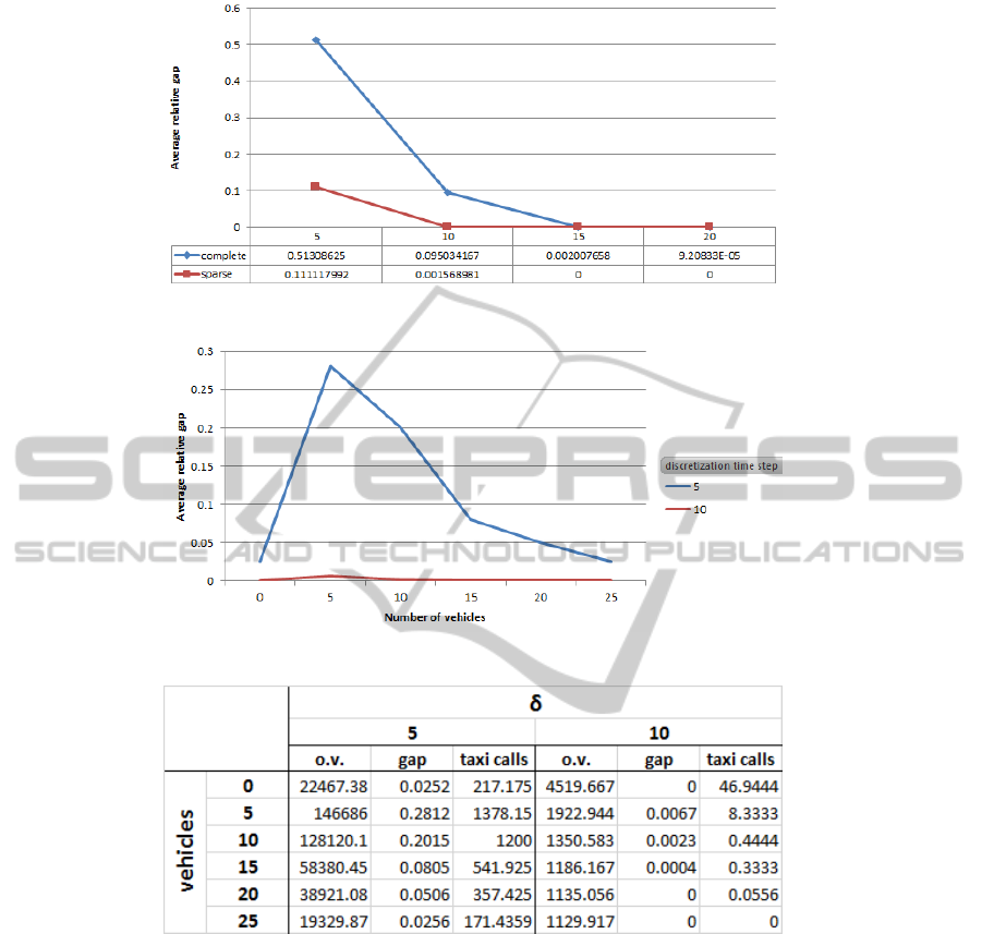
Figure 1: Dependence of Average Relative Gap on Number of Vehicles and Discretization Time Steps.

Figure 2: Dependence of Average Relative Gap on Number of Vehicles and Discretization Time Steps.

Figure 3: Dependence of Average Objective Function Value, Relative Gap and Number of Taxis on Number of Vehicles and

Discretization Time Steps.

4 CONCLUSION

In this paper, we address an important problem that

arises in the healthcare industry, that of transporting

laboratory samples between hospitals. This problem

arises because the laboratories within a hospital may

not be equipped to perform the required tests on a

sample. We present a mathematical programming for-

mulation of the problem, a solution procedure using

CPLEX, and a set of experiments to evaluate the so-

lution procedure. Even though we test our solution

procedure on generated data, we believe our solution

procedure can be used to solve the real-world problem

that motivated this exercise in the ﬁrst place. The ap-

proach outlined in this paper can be applied to solve

problems of comparable size that arise in the health-

care industry.

Future work may include a model-based heuris-

tic that will provide good solutions for larger problem

instances. In addition, the geographical area may be

partitioned into zones, and the size of the ﬂow net-

work reduced by removing arcs unlikely to be used

in an optimal solution. This may permit us to solve

much larger instances of the problem.

ANetworkModelfortheHospitalRoutingProblem

357

ACKNOWLEDGEMENTS

This research project has been supported by an

NSERC Discovery Grant awarded to Snezana Mitro-

vic Minic.

REFERENCES

Brønmo, G., Christiansen, M., Fagerholt, K., and Nygreen,

B. (2007). A multi-start local search heuristic for ship

scheduling - a computational study. In Computers &

Operations Research 34(1), pp 900-917.

Brysy, O. and Gendreau, M. (2005). Vehicle routing prob-

lem with time windows, part i: Route construction

and local search algorithms. In Transportation Sci-

ence 39(1), pp 104-118.

Ceder, A. (2003). Designing public transport network and

routes. In Advanced Modeling for Transit Operations

and Service Planning, W. H. K. Lam, M. G. H. Bell

(eds), pp 59-91. Emerald Group Publishing Limited,

Bingley.

Christiansen, M., Fagerholt, K., and Ronen, D. (2004). Ship

routing and scheduling: Status and perspectives. In

Transportation Science 38(1), pp 1-18.

Cordeau, J. F., Laporte, G., Savelsbergh, M. W. P., and Vigo,

D. (2007). Vehicle routing. In Transportation, Hand-

books in Operations Research and Management Sci-

ence, Volume 14, C. Barnhart and G. Laporte (eds),

pp 367-428. Elsevier, Amsterdam.

Cort

es, C. E., Matamala, M., and Contardo, C. (2010). The

pickup and delivery problem with transfers: Formu-

lation and a branch-and-cut solution method. In Eu-

ropean Journal of Operational Research 200, pp 711-

724.

Desrochers, M., Desrosiers, J., and Solomon, M. (1992).

A new optimization algorithm for the vehicle routing

problem with time windows. In Operations Research

40, pp 342-354.

Golden, B. L., Raghavan, S., and Wasil, E. A. (2008). The

vehicle routing problem: Latest advances and new

challenges. In Operations Research/Computer Sci-

ence Interfaces Series, Vol. 43. Springer.

Gopalan, R. and Talluri, K. T. (1998). Mathematical models

in airline schedule planning: A survey. In Annals of

Operations Research 76, pp 155-185.

Grasas, A., Ramalhinho, H., Pessoa, L. S., Resende, M.

G. C., Caball, I., and Barba, N. (2014). On the im-

provement of blood sample collection at clinical labo-

ratories. In BMC Health Services Research 14(12), 9

pages (DOI:10.1186/1472-6963-14-12).

Kallehauge, B., Larsen, J., Madsen, O. B. G., and Solomon,

M. M. (2005). Vehicle routing problem with time

windows. In Column Generation, G. Desaulniers, J.

Desrosiers, M. M. Solomon (eds), pp 67-98. Springer.

Karapetyan, D. and Punnen, A. P. (2013). A reduced integer

programming model for the ferry scheduling problem.

In Public Transport 4(3), pp 151-163.

Kohl, N., Desrosiers, J., Madsen, O. B. G., Solomon, M. M.,

and Soumis, F. (1999). 2-path cuts for the vehicle rout-

ing problem with time windows. In Transportation

Science 33(1), pp 101-116.

Kohl, N. and Madsen, O. B. G. (1997). An optimization

algorithm for the vehicle routing problem with time

windows based on lagrangian relaxation. In Opera-

tions Research 45(3), pp 395-406.

Laporte, G. (1992). The vehicle routing problem: An

overview of exact and approximate algorithms. In

European Journal of Operational Research 59(3), pp

345-358.

Laporte, G., Gendreau, M., Potvin, J.-Y., and Semet, F.

(2000). Classical and modern heuristics for the ve-

hicle routing problem. In International transactions

in operational research 7(4-5), pp 285-300.

Minic, S. M. (1998). Pickup and delivery problem with

time windows: A survey. In Simon Fraser University,

School of Computing Science, CMPT TR 1998-12.

Minic, S. M. and Laporte, G. (2006). The pickup and de-

livery problem with time windows and transshipment.

In INFOR 44(3), 217-227.

Minic, S. M. and Punnen, A. (2011). Scheduling of a het-

erogeneous ﬂeet of re-conﬁgurable ferries: a model, a

heuristic, and a case study. In OR 2011 - International

Conference on Operations Research, Zurich, Switzer-

land.

Rais, A. and Viana, A. (2010). Operations research in

healthcare: a survey. In International Transactions

in Operational Research 18, pp 1-31.

Savelsbergh, M. W. P. and Sol, M. (1995). The general

pickup and delivery problem. In Transportation Sci-

ence, 29 (1), pp 17-29.

Toth, P. and Vigo, D. (2002). The vehicle routing problem.

In SIAM.

ICORES2015-InternationalConferenceonOperationsResearchandEnterpriseSystems

358