Detection of Root Knot Nematodes in Microscopy Images
Faroq AL-Tam
1,2
, Ant
´
onio dos Anjos
3,4
, Stephane Bellafiore
5,6
and Hamid Reza Shahbazkia
1,7
1
Department of Electronic and Informatics Engineering, University of Algarve, Faro, Portugal
2
Faculty of Computer Science and Information Technology, University of Thamar, Dhamar, Yemen
3
ISMAT, Portim
˜
ao, Portugal
4
CCMAR-CIMAR Laborat
´
orio Associado, University of Algarve, 8005-139 Faro, Portugal
5
RPB, IRD Montpellier, France
6
LMI RICE, Hanoi, Vietnam
7
MIVEGEC, IRD Montpellier, France
Keywords:
Root Knot Nematodes, Vessel-like Detection, Illumination Correction, Thining, Mathematical Morphology.
Abstract:
Object detection in microscopy image is essential for further analysis in many applications. However, images
are not always easy to analyze due to uneven illumination and noise. In addition, objects may appear merged
together with debris. This work presents a method for detecting rice root knot nematodes in microscopy
images. The problem involves four subproblems which are dealt with separately. The uneven illumination
is corrected via polynomial fitting. The nematodes are then highlighted using mathematical morphology. A
binary image is obtained and the microscope lines are removed. Finally, the detected nematodes are counted
after thresholding the non-nematode particles. The results obtained from the performed tests show that this is
a reliable and effective method when compared to manual counting.
1 INTRODUCTION
Root Knot Nematodes (RKN) are plant parasitic mi-
croscopic animals responsible for a farm loss up to
$157 billion every year (Abad et al., 2008). All effi-
cient pesticides on RKN are not only toxic to humans
but also to the environment and have been banned re-
cently in most countries (M.B.T.O.Committee, 2010).
Pest management required an alternative. One
promising strategy is to find resistant plants that could
be crossed with interesting farmer crops to give a re-
sistant cultivar. However, breeding programs need the
ability of evaluating the plants’ resistance to the ne-
matode. To assess the resistance of a germplasm to
RKN, one should be able to exhaustively count the
offsprings’ number after a complete nematode life cy-
cle. But for microscopic parasites such as nematodes,
the process can be extremely time consuming and er-
ror prone. Counting objects under microscope for a
single plant takes around 15 to 30 minutes depend-
ing on the quantity of parasites. Moreover, the plant
breeder has to conscientiously observe the sample un-
der microscope to specifically count the number of
parasites. During the nematode sampling, several soil
and plant compounds are collected and can be misin-
terpreted as nematodes. To date, to our knowledge, no
software has been developed to assist plant breeders
in their resistance evaluation. Developing image pro-
cessing methods to allow the automation or semi au-
tomation of the counting process will drastically influ-
ence the precision and speed of these kind of experi-
ments and will allow faster experiment setups and bet-
ter results. This work describes an automatic method
for analyzing RKN in microscopy images.
2 THE PROPOSED APPROACH
This section addresses the technical details of the
problem and the proposed approach. In essence, four
different subproblems will be dealt with and solved.
These are:
1. Illumination correction.
2. Foreground detection.
3. Microscope lines suppression.
4. Nematode identification.
76
AL-Tam F., dos Anjos A., Bellafiore S. and Shahbazkia H..
Detection of Root Knot Nematodes in Microscopy Images.
DOI: 10.5220/0005209000760081
In Proceedings of the International Conference on Bioimaging (BIOIMAGING-2015), pages 76-81
ISBN: 978-989-758-072-7
Copyright
c
 2015 SCITEPRESS (Science and Technology Publications, Lda.)

2.1 Illumination Correction
Due to the variations in the light when acquiring the
images, illumination bias is recurrent in microscopy
imaging. In this work, the input images are con-
taminated by an uneven illumination field (Figure 1),
which has to be removed beforehand. To this end, the
input image is modeled by the multiplicative model as
(Young, 2001; Gonzalez and Woods, 2002):
S = T.B + ε (1)
Where the matrices S ∈ R
m×n
,T ∈ R
m×n
, and B ∈
R
m×n
, are the observed image, the true image, and the
bias field, respectively. “.” is the Hadamard element-
wise product, and ε ∈ R
m×n
is additive noise. Ob-
viously, (1) is an inverse ill-posed problem, because
the number of equations is lower than the number of
unknowns.
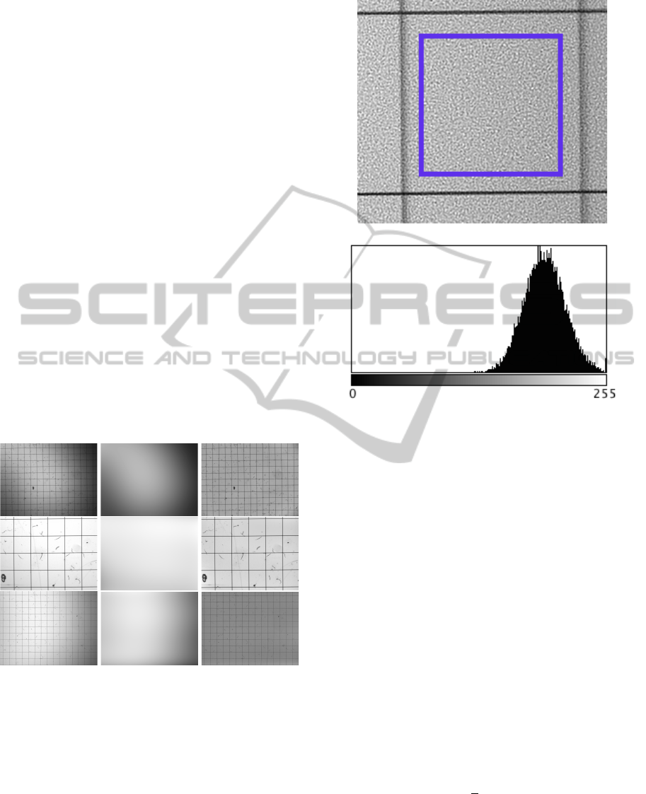
The input image can be enhanced by suppressing
the noise, simplifying Equation (1). The type of the
noise can be estimated by examining the distribution
of a clear (background only) region in the image. Fig-
ure 2b shows a clear Gaussian distribution as being
the histogram of the background image. For that rea-
son, the image is preprocessed by convolving it with
a Gaussian low pass filter with a kernel size k.
Figure 1: Illumination correction. Left: the input image,
middle: the estimated bias B, and right: the recovered image
T .
With the noise being removed, ε can be ignored
and (1) can be rewritten as:
log(S) = log(T ) + log(B) (2)
In (2), estimating B can be done in many different
ways. A comprehensive review can be found in (Hou,
2006; Vovk et al., 2007). Among these approaches,
surface fitting is suitable for this kind of images. This
type of images contain thin structures, therefore, a
proper 2-D smooth function can accurately model B
(a) A background region bounded by a rectangle.
(b) Respective intensity distribution
Figure 2: Identification of the noise type.
without including the objects in the estimated field. In
addition, estimating B by using a 2-D smooth function
reflects the main property of the illumination field, i.e.
B is assumed to be a slowly varying field.
B is modeled by using a bivariate polynomial of
degree d, where each pixel of B(x,y) is calculated as:
B(x,y;
~
θ,d) =
i=d
∑
i=0
j=i
∑
j=0
θ
i, j
x
i− j
y
j
(3)
which, in matrix form, can be rewritten as:
B = V
~
θ =



1 x
1
y
1
... x
i− j
1
y
j
1
.
.
.
.
.
.
.
.
.
.
.
.
.
.
.
1 x
r
y
r
... x
i− j
r
y
j
r



×






θ
0,0
θ
1,0
θ
1,1
.
.
.
θ
d,d






(4)
with r = mn. The problem of calculating B from
(2), boils down to a least squares problem of estimat-
ing the vector of parameters
~
θ as:
argmin
~
θ
1
2
kV
~
θ −
~
sk
2
2
(5)
where
~
s is a vector created by concatenating the
columns of S.
~
θ can be therefore found by the normal
equations as:
~
θ = (V
>
V )
−1
V
>
~
s (6)
DetectionofRootKnotNematodesinMicroscopyImages
77

Examples of applying the illumination correction
are shown in Figure 1.
2.2 Foreground Detection
In some situations, general thresholding approaches,
like iso-data (Trussell, 1978), Otsu (Otsu, 1975), and
local-mean (Fisher R., 1996) may be suitable for de-
tecting the foreground. However, such methods are
general, in the sense that they statistically estimate a
threshold that separates two classes in the image data.
In other words, they use zero knowledge about the
shape of the objects to be detected. These methods
even if success to segment the image, they will de-
tect all objects regardless of their shape. In this work,
only elongated objects are targeted, therefore, the de-
tection of the nematodes is two-fold. First, thin struc-
tures are highlighted. Second, the resulting image is
segmented in order to obtain a binary version.
2.2.1 Detection of Thin Structures
The detection of thin and vessel-like structures is
a popular problem, especially in the medical and
microscopy image analysis community. For this
purpose, different approaches have been developed.
Examples include, Frangi’s method (Frangi et al.,
1998), differential geometry (Steger, 1998), matched
filters (Chaudhuri et al., 1989), mathematical mor-
phology (MM) (Zana and Klein, 2001), and tracing
methods (Yim et al., 2000; Meijering et al., 2004).
An approach using mathematical morphology (MM)
(Figueiredo and Leitao, 1995) is chosen due to two
reasons. First, most of the other methods have re-
sponses at the object’s edges, which is not desirable.
Second, MM is computationally efficient.
In MM the input image can be looked at as a to-
pographic surface. A nematode can be seen as a nar-
row continuous plateau with minima spanning its me-
dial line. Here the input image is grayscale with dark
objects and light background, and the structuring ele-
ments (SE) is flat. A great advantage in MM is that al-
most all filters are made of two basic building blocks:
erosion and dilation (Serra, 1983). The grayscale flat
dilation of the image T by the structuring element f
is defined as:
T ⊕ f = max
a,b∈ f
T (x + a, y + b) (7)
Similarly, the flat erosion is defined as:
T  f = min
a,b∈ f
T (x + a, y + b) (8)
These two operators are very common and easy
to implement as they can be conceived as minimum
(for erosion) and maximum (for dilation) filters. In-
side a region defined by the geometry of the f (e.g. a
disk), each pixel of the image is replaced by either the
maximum or the minimum neighbor according to the
operator type (Figueiredo and Leitao, 1995).
Using these two basic operators, additional filters
can be built. Another two popular operators are open
and close. Opening is defined as the erosion followed
by dilation:
T ◦ f = (T  f ) ⊕ f (9)
Likewise, mathematical closing is defined as dila-
tion of erosion:
T • f = (T ⊕ f )  f (10)
For detecting elevations, two specialized operators
can be used: top-hat and bottom-hat transforms. A
top-hat transform is defined as the difference between
the image and an opened version of itself.
τ
top
(T, f ) = T − (T ◦ f ) (11)
The bottom-hat transform is the difference between
the image and a closed version.
τ
bottom
(T, f ) = T − (T • f ) (12)
Due to the nice property of the top/bottom-hat
transforms of highlighting specific features, they were
used in many vessel-like structure detection methods
e.g. (Zana and Klein, 2001; Mendonc¸a and Campilho,
2006). When an appropriate radius of f is selected,
the foreground pixels can be highlighted and the back-
ground artifacts can be reduced. Given a flat disk
structuring element f , with radius ϑ. The recovered
image T is transformed by the bottom-hat operator as
in (12). The results of detecting the foreground are
shown in Figure 3.
2.2.2 Segmentation
To threshold the response of the bottom-hat trans-
form, let µ be the mean of the image τ
bottom
(T, f ).
The binary image is obtained as:
T
binary
=

255 if τ
bottom
(T, f ) ≤ µ
0 otherwise
(13)
The result of segmentation is shown in Figure 3.
2.3 Microscope Lines Suppression
With the presence of the microscope lines, it is very
difficult to detect the intended objects. The nema-
tode counting cells are provided with carved micro-
scope lines offering the investigator access to a pre-
cise volume unit (here, the number of nematodes per
BIOIMAGING2015-InternationalConferenceonBioimaging
78

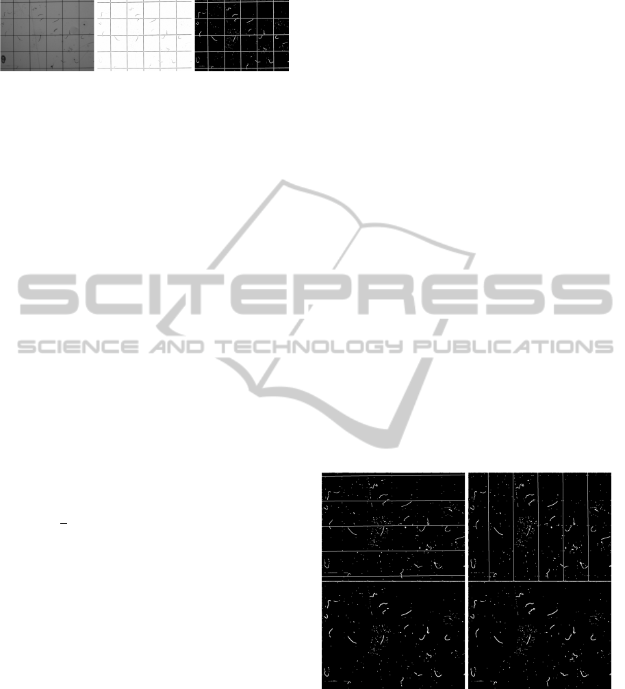
Figure 3: Detection of the nematodes using the bottom-hat
transform. Left: a sample image. Middle: the response of
the bottom-hat transform of a disk structuring element with
radius 5. Right: the resulting binary image.
volume unit). In other words, a counting chamber
needs to have these lines to define a volume unit, and
nematologists count particles with these lines. How-
ever those microscope lines cannot be removed by
the investigator as this would modify the volume unit
and thereby lose precision. Furthermore, these lines
have approximately the same width as the nematodes,
which makes the detection task even harder. The re-
moval of the lines is not trivial, because there are in-
tersections between them and the nematodes. There-
fore, there has to be a reconnecting approach for ne-
matodes being split.
In order to remove the lines, the Euclidean dis-
tance map T
EDM
(Meijster et al., 2002) and the skele-
ton T
skeleton
(Zhang and Suen, 1984) of T
binary
are
calculated. Before removing a line, it is impor-
tant to know its width. Let a connected component
in T
binary
be denoted by the set of points P. Let
SKELETON(P) ⊆ P be the set of skeleton points of
the component P. As these lines correspond to the
maximum connected component (P
max
) in T
binary
, the
radius ρ of the lines is calculated as:
ρ(P
max
) =
1
z
z
∑
i=1
EDM(p
i
), ∀p ∈ SKELETON(P
max
)
(14)
where z is the size of SKELETON(P
max
).
As the lines are only horizontal and vertical, the
skeleton image is convolved by these line detection
kernels:
h
horizontal
=


−1 −1 −1
2 2 2
−1 −1 −1


(15)
h
vertical
=


−1 2 −1
−1 2 −1
−1 2 −1


(16)
In the beginning, the skeleton image T
skeleton
is
convolved by the h
horizontal
in order to detect the hori-
zontal lines. The region of radius ρ(P
max
) centered at
each one of these lines is suppressed all the way along
each line. In order to avoid removing the nematodes
that are horizontal, a length threshold ` is used to re-
move any horizontal line with length ≥ `. The same
process is repeated with h
vertical
to detect and suppress
the vertical lines. The result of this process is an im-
age without lines T
clean
(Figure 4).
2.4 Nematodes Identification
During the suppression of the lines, some nematodes
are being split. They are rejoined by using a search
approach. The detected horizontal lines from T
skeleton
are scanned against the T
binary
by passing a vertical
line of length 2 ∗ ρ(P
max
) + c at each point of the hor-
izontal line. Where c is a small integer (e.g. 2). If
all the points of this small vertical line belong to the
foreground of T
binary
, foreground pixels (i.e. 255) are
added in the position of this vertical line to the T
clean
image. The same process is adapted for the vertical
lines detected in T
skeleton
, but using a small horizontal
line with the length 2 ∗ ρ(P
max
)+ c as well. The result
is an image with the unsplit detected nematodes. In
order to filter out the detected debris, the medial axis
of each detected object is cleaned by removing skele-
ton branches of length ≤ 2 ∗ ρ(P
max
) (i.e. to smooth
the skeleton). This helps to establish a thresholding
approach based on the length of the medial axis to
differentiate nematodes from other objects. There-
fore, among the detected objects, only the ones with
length ≥ u are identified as nematodes. The accuracy
of the proposed method was computed by comparing
the number of detected nematodes to the number of
nematodes existing in a ground truth.
Figure 4: Line detection and suppression. Top row: detect-
ing the horizontal and vertical lines. Bottom row: rejoining
the splitted nematodes.
3 RESULTS
To evaluate the described method, a set of 12
grayscale nematode images were used. Each image
size is 2048×1536. The method was compared to a
DetectionofRootKnotNematodesinMicroscopyImages
79

ground truth (GT) of manually counted nematodes.
These results are shown in Table 1. The parame-
ters used in this test are shown in Table 2. The de-
tected (Det.) nematodes were evaluated in terms of
True Positive (TP), False Positive (FP), False Neg-
ative (FN), Positive Predictive Value (PPV)
T P
T P+FP
,
and Recall
T P
T P+FN
.
Table 1: Nematode detection results of 12 samples.
# GT Det. TP FP FN PPV Recall
1 71 66 66 0 5 1.00 0.93
2 75 87 70 17 5 0.80 0.93
3 45 62 45 17 0 0.73 1.00
4 38 42 34 8 4 0.81 0.89
5 33 37 28 9 5 0.76 0.85
6 32 35 30 5 2 0.86 0.94
7 15 17 14 3 1 0.82 0.93
8 21 26 19 7 2 0.73 0.90
9 45 40 36 4 9 0.90 0.80
10 66 59 57 2 9 0.97 0.86
11 39 42 36 6 3 0.86 0.92
12 36 36 36 0 0 1.00 1.00
Table 2: The parameters used (measured in pixels).
Parameter Description Value
k Gaussian kernel radius 3
` Min. length of a line 0.3m
ϑ Bottom hat transform radius 5
u Min. length of a nematode 30
The averages of PPV and Recall where ≈ 0.85 and
≈ 0.91, respectively. The FN is low which indicating
that the proposed approach performed a good detec-
tion. Most of the time the missed nematodes were al-
most hidden by the microscope lines or partially vis-
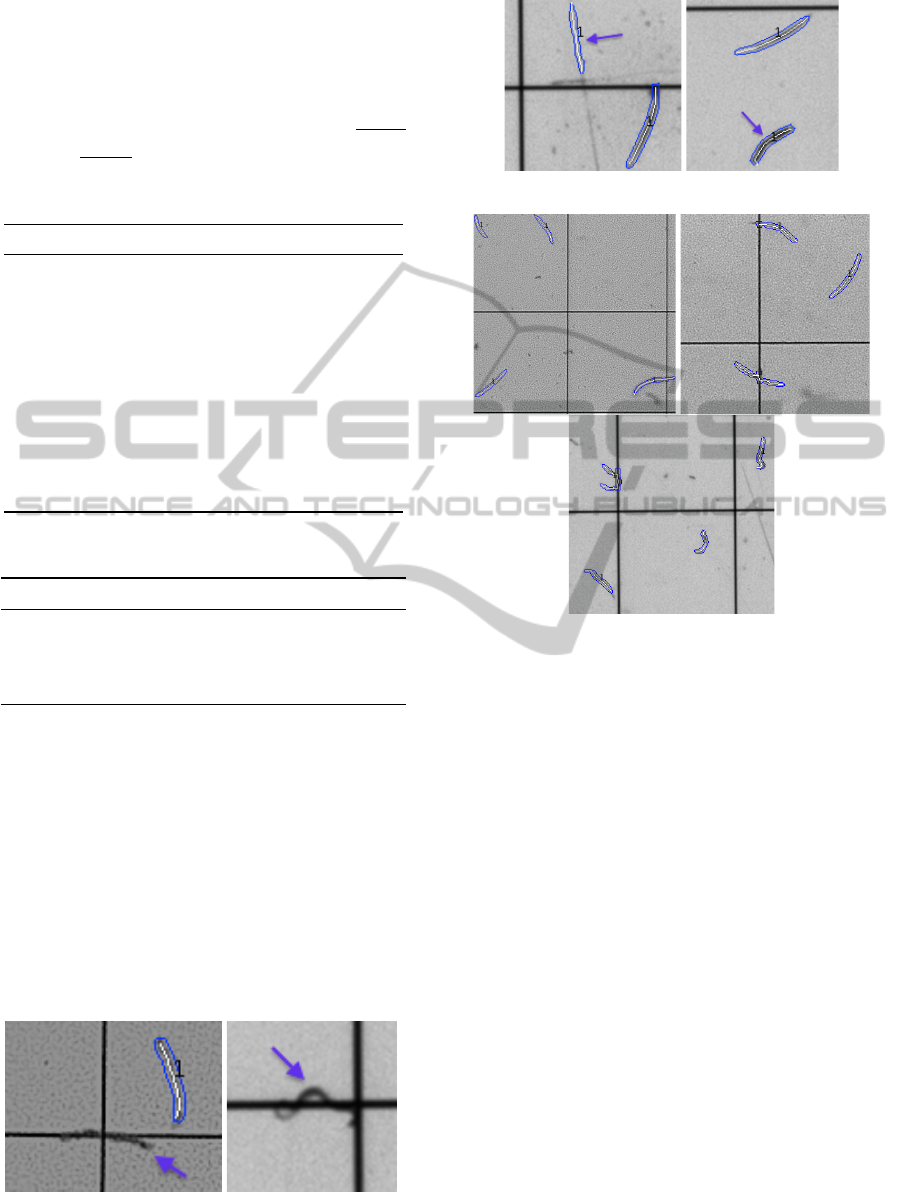
ible (Figure 5). However, in some cases, there were
nematode-like artifacts which increased the number
of FP. An example of this kind of non-desirable arti-
facts is shown in Figure 6. Overall, the method looks
very promising and shows reliable results, especially,
when it comes to images that do not contain unwanted
nematode-like artifacts (Figure 7).
Figure 5: Examples of missed nematodes due to partial vis-
ibility (pointed by the arrow).
Figure 6: Nematode-like objects (pointed by the arrow).
Figure 7: Examples of nematodes detected by the proposed
approach.
4 CONCLUSION
A method for Root Knot Nematode detection in mi-
croscopy images was presented. The input images
suffered from uneven illumination and noise contam-
ination. The noise was suppressed by a Gaussian fil-
ter and, then, the illumination was corrected by 2-
D polynomial fitting. The mathematical morphology
bottom-hat transform is used afterwards to highlight
the nematodes. A binary image is obtained by thresh-
olding the response of the bottom-hat. Two filters
were used to remove the microscope lines from the
binary image. Nematodes being split due to the lines’
suppression were merged by a search method. The
final quantification results were collected based on a
length threshold of the detected object medial axis.
The experimental results showed a reliable detection
when comparing the method to a manually created
ground truth. To evaluate the offsprings’ number,
classical counting techniques require the presence of
one or several researchers in front of their microscope
all day long. Mistakes are bound to occur, leading to
a misevaluation of the offsprings’ number. To bypass
this artifact the only solution is to increase the sam-
BIOIMAGING2015-InternationalConferenceonBioimaging
80

ple number to obtain statistical significance. How-
ever, by doing so, the evaluation time significantly
increases. As most laboratories can generate images
with a camera linked to a microscope, we believe that
our method can be easily extended to their structures
offering a fast and reproducible technique. This ap-
proach will make way for the development of a plat-
form allowing high throughput selection of plant re-
sistant cultivars. Moreover, beside the direct interest
of breeders to this kind of tool, our approach could
also be of interest to other biological fields. Indeed,
it is possible to measure the number of nematodes per
volume unit but also to assess the size of each ne-
matode providing access to traits that could be very
informative to ecology studies.
ACKNOWLEDGEMENTS
This work was partially financed by SPIRALE and
MENERGEP (GRiSP) projects, IRD Montpellier
France. We also acknowledge the INFECTOPOL
SUD Marseille France for granting the cooperation.
REFERENCES
Abad, P., Gouzy, J., Aury, J.-M., Castagnone-Sereno, P.,
Danchin, E. G., Deleury, E., Perfus-Barbeoch, L., An-
thouard, V., Artiguenave, F., Blok, V. C., et al. (2008).
Genome sequence of the metazoan plant-parasitic ne-
matode meloidogyne incognita. Nature biotechnol-
ogy, 26(8):909–915.
Chaudhuri, S., Chatterjee, S., Katz, N., Nelson, M., and
Goldbaum, M. (1989). Detection of blood vessels in
retinal images using two-dimensional matched filters.
Medical Imaging, IEEE Transactions on, 8(3):263–
269.
Figueiredo, M. A. and Leitao, J. M. (1995). A nonsmooth-
ing approach to the estimation of vessel contours in
angiograms. Medical Imaging, IEEE Transactions on,
14(1):162–172.
Fisher R., Perkins S., W. A. . W. E. (1996.). Hypermedia
Image Processing Reference. J. Wiley & Sons Pub-
lishing.
Frangi, A. F., Niessen, W. J., Vincken, K. L., and Viergever,
M. A. (1998). Multiscale vessel enhancement filter-
ing. In Medical Image Computing and Computer-
Assisted Interventation - MICCAI 98, pages 130–137.
Springer.
Gonzalez, R. C. and Woods, R. E. (2002). Digital Image
Processing, 2-nd Edition. Prentice Hall.
Hou, Z. (2006). A review on mr image intensity inhomo-
geneity correction. International Journal of Biomedi-
cal Imaging, 2006.
M.B.T.O.Committee (2010). 2010 report of the methyl bro-
mide technical options committee 2010 assessment.
Technical report, Nairobi, United Nations Environ-
ment Program (UNEP).
Meijering, E., Jacob, M., Sarria, J.-C., Steiner, P., Hirling,
H., and Unser, M. (2004). Design and validation of a
tool for neurite tracing and analysis in fluorescence
microscopy images. Cytometry Part A, 58(2):167–
176.
Meijster, A., Roerdink, J. B., and Hesselink, W. H. (2002).
A general algorithm for computing distance trans-
forms in linear time. In Mathematical Morphology
and its applications to image and signal processing,
pages 331–340. Springer.
Mendonc¸a, A. M. and Campilho, A. (2006). Segmenta-
tion of retinal blood vessels by combining the detec-
tion of centerlines and morphological reconstruction.
Medical Imaging, IEEE Transactions on, 25(9):1200–
1213.
Otsu, N. (1975). A threshold selection method from gray-
level histograms. Automatica, 11(285-296):23–27.
Serra, J. (1983). Image analysis and mathematical morphol-
ogy.
Steger, C. (1998). An unbiased detector of curvilinear
structures. Pattern Analysis and Machine Intelligence,
IEEE Transactions on, 20(2):113–125.
Trussell, H. J. (1978). Picture thresholding using an itera-
tive selection method. Systems, Man and Cybernetics,
IEEE Transactions on, 8(8):630–632.
Vovk, U., Pernus, F., and Likar, B. (2007). A review
of methods for correction of intensity inhomogene-
ity in mri. Medical Imaging, IEEE Transactions on,
26(3):405–421.
Yim, P. J., Choyke, P. L., and Summers, R. M. (2000). Gray-
scale skeletonization of small vessels in magnetic res-
onance angiography. Medical Imaging, IEEE Trans-
actions on, 19(6):568–576.
Young, I. T. (2001). Shading Correction: Compensation for
Illumination and Sensor Inhomogeneities. John Wiley
& Sons, Inc.
Zana, F. and Klein, J.-C. (2001). Segmentation of vessel-
like patterns using mathematical morphology and cur-
vature evaluation. Image Processing, IEEE Transac-
tions on, 10(7):1010–1019.
Zhang, T. Y. and Suen, C. Y. (1984). A fast parallel algo-
rithm for thinning digital patterns. Commun. ACM,
27(3):236–239.
DetectionofRootKnotNematodesinMicroscopyImages
81