An Online Vector Error Correction Model for Exchange Rates

Forecasting

Paola Arce

, Jonathan Antognini

, Werner Kristjanpoller

and Luis Salinas

1,3

Departamento de Inform

atica, Universidad T

ecnica Federico Santa Mar

ıa, Valpara

ıso, Chile

Departamento de Industrias, Universidad T

ecnica Federico Santa Mar

ıa, Valpara

ıso, Chile

CCTVal, Universidad T

ecnica Federico Santa Mar

ıa, Valpara

ıso, Chile

Keywords:

Vector Error Correction Model, Online Learning, Financial Forecasting, Foreign Exchange Market.

Abstract:

Financial time series are known for their non-stationary behaviour. However, sometimes they exhibit some

stationary linear combinations. When this happens, it is said that those time series are cointegrated.The Vector

Error Correction Model (VECM) is an econometric model which characterizes the joint dynamic behaviour

of a set of cointegrated variables in terms of forces pulling towards equilibrium. In this study, we propose an

Online VEC model (OVECM) which optimizes how model parameters are obtained using a sliding window of

the most recent data. Our proposal also takes advantage of the long-run relationship between the time series

in order to obtain improved execution times. Our proposed method is tested using four foreign exchange rates

with a frequency of 1-minute, all related to the USD currency base. OVECM is compared with VECM and

ARIMA models in terms of forecasting accuracy and execution times. We show that OVECM outperforms

ARIMA forecasting and enables execution time to be reduced considerably while maintaining good accuracy

levels compared with VECM.

1 INTRODUCTION

In ﬁnance, it is common to ﬁnd variables with long-

run equilibrium relationships. This is called cointe-

gration and it reﬂects the idea of that some set of vari-

ables cannot wander too far from each other. Coin-

tegration means that one or more linear combinations

of these variables are stationary even though individ-

ually they are not (Engle and Granger, 1987). Fur-

thermore, the number of cointegration vectors reﬂects

how many of these linear combinations exist. Some

models, such as the Vector Error Correction (VECM),

take advantage of this property and describe the joint

behaviour of several cointegrated variables.

VECM introduces this long-run relationship

among a set of cointegrated variables as an error cor-

rection term. VECM is a special case of the vector

autorregresive model (VAR) model. VAR model ex-

presses future values as a linear combination of vari-

ables past values. However, VAR model cannot be

used with non-stationary variables. VECM is a lin-

ear model but in terms of variable differences. If

cointegration exists, variable differences are station-

ary and they introduce an error correction term which

adjusts coefﬁcients to bring the variables back to equi-

librium. In ﬁnance, many economic time series are

revealed to be stationary when they are differentiated

and cointegration restrictions often improves fore-

casting (Duy and Thoma, 1998). Therefore, VECM

has been widely adopted.

In ﬁnance, pair trading is a very common exam-

ple of cointegration application (Herlemont, 2003)

but cointegration can also be extended to a larger set

of variables (Mukherjee and Naka, 1995),(Engle and

Patton, 2004).

Both VECM and VAR model parameters are ob-

tained using ordinary least squares (OLS) method.

Since OLS involves many calculations, the parame-

ter estimation method is computationally expensive

when the number of past values and observations in-

creases. Moreover, obtaining cointegration vectors is

also an expensive routine.

Recently, online learning algorithms have been

proposed to solve problems with large data sets be-

cause of their simplicity and their ability to update

the model when new data is available. The study pre-

sented by (Arce and Salinas, 2012) applied this idea

using ridge regression.

There are several popular online methods

such as perceptron (Rosenblatt, 1958), passive-

193

Arce P., Antognini J., Kristjanpoller W. and Salinas L..

An Online Vector Error Correction Model for Exchange Rates Forecasting.

DOI: 10.5220/0005205901930200

In Proceedings of the International Conference on Pattern Recognition Applications and Methods (ICPRAM-2015), pages 193-200

ISBN: 978-989-758-077-2

 2015 SCITEPRESS (Science and Technology Publications, Lda.)

aggressive (Crammer et al., 2006), stochastic gradient

descent (Zhang, 2004), aggregating algorithm (Vovk,

2001) and the second order perceptron (Cesa-Bianchi

et al., 2005). In (Cesa-Bianchi and Lugosi, 2006), an

in-deph analysis of online learning is provided.

In this paper, we propose an online formulation of

the VECM called Online VECM (OVECM). OVECM

is a lighter version of VECM which considers only a

sliding window of the most recent data and introduces

matrix optimizations in order to reduce the number of

operations and therefore execution times. OVECM

also takes into account the fact that cointegration vec-

tor space doesn’t experience large changes with small

changes in the input data.

OVECM is later compared against VECM and

ARIMA models using four currency rates from the

foreign exchange market with 1-minute frequency.

VECM and ARIMA models were used in an itera-

tive way in order to allow fair comparison. Execu-

tion times and forecast performance measures MAPE,

MAE and RMSE were used to compare all methods.

Model effectiveness is focused on out-of-sample

forecast rather than in-sample ﬁtting. This criteria

allows the OVECM prediction capability to be ex-

pressed rather than just explaining data history.

The next sections are organized as follows: sec-

tion 2 presents the VAR and VECM, the OVECM al-

gorithm proposed is presented in section 3. Section 4

gives a description of the data used and the tests car-

ried on to show accuracy and time comparison of our

proposal against the traditional VECM and section 5

includes conclusions and a proposal for future study.

2 BACKGROUND

2.1 Integration and Cointegration

A time series y is said to be integrated of order d if

after differentiating the variable d times, we get an

I(0) process, more precisely:

(1 − L)

y ∼ I(0) ,

where I(0) is a stationary time series and L is the lag

operator:

(1 − L)y = ∆y = y

− y

t−1

∀t

Let y

= {y

, . . . , y

} be a set of l stationary time

series I(1) which are said to be cointegrated if a vector

β = [β(1), . . . , β(l)]

∈ R

exists such that the time

series,

:= β

= β(1)y

+ ··· + β(l)y

∼ I(0). (1)

In other words, a set of I(1) variables is said to

be cointegrated if a linear combination of them exists

which is I(0).

2.2 Vector Autorregresive Models

VECM is a special case of VAR model and both de-

scribe the joint behaviour of a set of variables.

VAR(p) model is a general framework to describe

the behaviour of a set of l endogenous variables as

a linear combination of their last p values. These l

variables at time t are represented by the vector y

follows:



1,t

2,t

. . . y

l,t



where y

j,t

corresponds to the time series j evaluated

at time t.

The VAR(p) model describes the behaviour of a

dependent variable in terms of its own lagged values

and the lags of the others variables in the system. The

model with p lags is formulated as the following:

= φ

t−1

+ ··· + φ

t−p

+ c + ε

, (2)

where t = p + 1, . . . N, φ

, . . . , φ

are l × l matrices of

real coefﬁcients, ε

p+1

, . . . , ε

are error terms, c is a

constant vector and N is the total number of samples.

The VAR matrix form of equation (2) is:

B = AX + E , (3)

where:

A =







. . . y

N−1

p−1

. . . y

N−2

. . . y

N−p

1 . . . 1







B =





p+1

. . . y





X =





··· φ





E =





p+1

. . . ε





Equation (3) can be solved using ordinary least

squares estimation.

ICPRAM2015-InternationalConferenceonPatternRecognitionApplicationsandMethods

194

2.3 VECM

VECM is a special form of a VAR model for I(1) vari-

ables that are also cointegrated (Banerjee, 1993). It

is obtained by replacing the form ∆y

= y

− y

t−1

equation (2). VECM is expressed in terms of differ-

ences, has an error correction term and the following

form:

∆y

= Ωy

t−1

| {z }

Error correction term

p−1

∑

i=1

∗

∆y

t−i

+ c + ε

, (4)

where coefﬁcients matrices Ω and φ

∗

are function of

matrices φ

(shown in equation (2)) as follows:

∗

:= −

∑

j=i+1

Ω := −(I − φ

− ··· − φ

)

The matrix Ω has the following properties (Johansen,

1995):

• If Ω = 0 there is no cointegration

• If rank(Ω) = l i.e full rank, then the time series

are not I(1) but stationary

• If rank(Ω) = r, 0 < r < l then, there is coin-

tegration and the matrix Ω can be expressed as

Ω = αβ

, where α and β are (l × r) matrices and

rank(α) = rank(β) = r.

The columns of β contains the cointegration vec-

tors and the rows of α correspond with the ad-

justed vectors. β is obtained by Johansen proce-

dure (Johansen, 1988) whereas α has to be deter-

mined as a variable in the VECM.

It is worth noticing that the factorization of the

matrix Ω is not unique since for any r × r nonsin-

gular matrix H we have:

αβ

= αHH

−1

= (αH)(β(H

−1

)

= α

∗

(β

∗

)

with α

∗

= αH and β

∗

= β(H

−1

)

If cointegration exists, then equation (4) can be

written as follows:

∆y

= αβ

t−1

p−1

∑

i=1

∗

∆y

t−i

+ c + ε

which is a VAR model but for time series differences.

VECM has the same form shown in equation (3)

but with different matrices:

A =







··· β

N−1

∆y

··· ∆y

N−1

∆y

··· ∆y

N−p+1

1 ··· 1







, (5)

B =





∆y

p+1

. . . ∆y





, (6)

X =





α φ

∗

··· φ

∗

p−1





, (7)

E =





p+1

. . . ε





(8)

VAR and VECM parameters shown in equation

(3) can be solved using standard regression tech-

niques, such as ordinary least squares (OLS).

2.4 Ordinary Least Squares Method

When A is singular, solution to equation (3) is given

by the ordinary least squares (OLS) method. OLS

consists of minimizing the sum of squared errors or

equivalently minimizing the following expression:

min

kAX − Bk

for which the solution

X is well-known:

X = A

where A

is the Moore-Penrose pseudo-inverse which

can be written as follows:

= (A

−1

. (9)

However, when A is not full rank, i.e rank(A) =

k < n ≤ m, A

A is always singular and equation (9)

cannot be used. More generally, the pseudo-inverse is

best computed using the compact singular value de-

composition (SVD) of A:

m×n

= U

m×k

k×k

k×n

as follows

= V

−1

AnOnlineVectorErrorCorrectionModelforExchangeRatesForecasting

195

3 METHODOLOGY

3.1 Online VECM

Since VECM parameter estimation is computation-

ally expensive, we propose an online version of

VECM (OVECM). OVECM considers only a slid-

ing window of the most recent data. Moreover, since

cointegration vectors represent long-run relationships

which vary little in time, OVECM determines ﬁrstly

if they require calculation.

OVECM also implements matrix optimizations in

order to reduce execution time, such as updating ma-

trices with new data, removing old data and introduc-

ing new cointegration vectors.

Algorithm 1 shows our OVECM proposal which

considers the following:

• The function getJohansen returns cointegration

vectors given by the Johansen method considering

the trace statistic test at 95% signiﬁcance level.

• The function vecMatrix returns the matrices (5)

and (6) that allows VECM to be solved.

• The function vecMatrixOnline returns the ma-

trices (5) and (6) aggregating new data and remov-

ing the old one, avoiding calculation of the matrix

A from scratch.

• Out-of-sample outputs are saved in the variables

true

and Y

pred

• The model is solved using OLS.

• In-sample outputs are saved in the variables ∆y

true

and ∆y

pred

• The function mape gets the in-sample MAPE for

the l time series.

• Cointegration vectors are obtained at the begin-

ning and when they are required to be updated.

This updating is decided based on the in-sample

MAPE of the last n inputs. The average of all

MAPEs are stored in the variable e. If the aver-

age of MAPEs (mean(e)) is above a certain error

given by the mean error threshold, cointegration

vectors are updated.

• If new cointegration vectors are required, the

function vecMatrixUpdate only updates the cor-

responding columns of matrix A affected by those

vectors (see equation 5).

Our proposal was compared against VECM and

ARIMA. Both algorithms were adapted to an online

context in order to get a reasonable comparison with

our proposal (see algorithms 2 and 3). VECM and

ARIMA are called with a sliding window of the most

Algorithm 1: OVECM: Online VECM.

Input:

y: matrix with N input vectors and l time series

p: number of past values

L: sliding window size (L < N)

mean error: MAPE threshold

n: interpolation points to obtain MAPE

Output:

pred

[L + 1], . . . , y

pred

[N]}: model predictions

1: for i = 0 to N − L do

2: y

← y[i : i + L]

3: if i = 0 then

4: v ← getJohansen(y

, p)

5: [A B] ← vecMatrix(y

, p, v)

6: else

7: [A B] ← vecMatrixOnline(y

, p, v, A, B)

8: ∆Y

pred

[i] ← A[−1, :] × X

9: end if

10: X ← OLS(A, B)

11: e ← mape(B[−n, :], A[−n, :] × X)

12: if mean(e) > mean error then

13: v ← getJohansen(y

, p)

14: A ← vecMatrixUpdate(y

, p, v, A)

15: X ← OLS(A, B)

16: end if

17: end for

18: Y

true

← Y[L + 1 : N]

19: Y

pred

← Y[L : N − 1] + ∆Y

pred

Algorithm 2: SLVECM: Sliding window VECM.

Input:

y: matrix with N input vectors and l time series

p: number of past values

L: sliding window size (L < N)

Output:

pred

[L + 1], . . . , y

pred

[N]}: model predictions

1: for i = 0 to N − L do

2: y

← y[i : i + L + 1]

3: model = V ECM(y

, p)

4: Y

pred

[i] = model.predict(y[i + L])

5: end for

6: Y

true

= y[i + L + 1 : N]

recent data, whereby the models are updated at every

time step.

Since we know out time series are I(1) SLARIMA

is called with d = 1. ARIMA is executed for every

time series.

Both OVECM and SLVECM time complexity

is dominated by Johansen method which is O(n

Thus, both algorithms order is O(Cn

) where C is the

number of iterations.

ICPRAM2015-InternationalConferenceonPatternRecognitionApplicationsandMethods

196

Algorithm 3: SLARIMA: Sliding window ARIMA.

Input:

y: matrix with N input vectors and l time series

p: autoregressive order

d: integrated order

q: moving average order

L: sliding window size (L < N)

Output:

pred

[L + 1], . . . , y

pred

[N]}: model predictions

1: for i = 0 to N − L do

2: for j = 0 to l − 1 do

3: y

← y[i : i + L + 1, j]

4: model = ARIMA(y

, (p, d, q))

5: Y

pred

[i, j] = model.predict(y[i + L, j])

6: end for

7: end for

8: Y

true

= y[i + L + 1 : N, :]

3.2 Evaluation Methods

Forecast performance is evaluated using different

methods. We have chosen three measures usually

used:

MAPE. Mean Average Percent Error which presents

forecast errors as a percentage.

MAPE =

∑

t=1

−

× 100 (10)

MAE. Mean Average Error which measures the dis-

tance between forecasts to the true value.

MAE =

∑

t=1

−

(11)

RMSE. Root Mean Square Error also measures the

distance between forecasts to the true values but,

unlike MAE, large deviations from the true value

have a large impact on RMSE due to squaring

forecast error.

RMSE =

∑

t=1

−

)

(12)

3.3 Model Selection

Akaike Information Criterion (AIC) is often used in

model selection where AIC with smaller values are

preferred since they represent a trade-off between bias

and variance. AIC is obtained as follows:

AIC = −

bias

variance

(13)

where

l is the loglikelihood function

k number of estimated parameters

N number of observations

Loglikelihood function is obtained from the

Residual Sum of Squares (RSS):

l = −



1 + ln(2π) + ln



RSS



(14)

4 RESULTS

4.1 Data

Tests of SLVECM, SLARIMA and our proposal

OVECM were carried out using foreign four ex-

change data rates: EURUSD, GBPUSD, USDCHF

and USDJPY. This data was collected from the free

database Dukascopy which gives access to the Swiss

Foreign Exchange Marketplace (Dukascopy, 2014).

The reciprocal of the last two rates (CHFUSD,

JPYUSD) were used in order to obtain the same

base currency for all rates. The tests were done us-

ing 1-minute frequency from ask prices which corre-

sponded to 1.440 data points per day from the 11th to

the 15th of August 2014.

4.2 Unit Root Tests

Before running the tests, we ﬁrstly checked if they

were I(1) time series using the Augmented Dickey

Fuller (ADF) test.

Table 1: Unit roots tests.

Statistic Critical value Result

EURUSD -0.64 -1.94 True

∆EURUSD -70.45 -1.94 False

GBPUSD -0.63 -1.94 True

∆GBPUSD -54.53 -1.94 False

CHFUSD -0.88 -1.94 True

∆CHFUSD -98.98 -1.94 False

JPYUSD -0.65 -1.94 True

∆JPYUSD -85.78 -1.94 False

Table 1 shows that all currency rates cannot reject

the unit root test but they rejected it with their ﬁrst

differences. This means that all of them are I(1) time

series and we are allowed to use VECM and therefore

OVECM.

AnOnlineVectorErrorCorrectionModelforExchangeRatesForecasting

197

4.3 Parameter Selection

In order to set OVECM parameters: windows size L

and lag order p, we propose to use several window

sizes: L = 100, 400, 700, 1000. For every window size

L we chose lag order with minimum AIC.

ARIMA parameters were also obtained using

AIC. Parameters optimization is presented in table 2:

Table 2: Parameters optimization. VECM order and

ARIMA parameters were selected using AIC.

Windows size L VECM ARIMA

L order (p) order (p, d, q)

100 2 p=2,d=1,q=1

400 5 p=1,d=1,q=1

700 3 p=2,d=1,q=1

1000 3 p=2,d=1,q=1

In OVECM we also deﬁne a mean error vari-

able, which was deﬁned based on the in-sample

MAPEs. Figure 1 shows how MAPE moves and how

mean error variable help us to decide whether new

cointegration vectors are needed.

Figure 1: In-sample MAPEs example for 50 minutes. The

average of them is considered to obtain new cointegration

vectors.

4.4 Execution Times

We ran OVECM and SLVECM 400 iterations.

SLARIMA execution time is excluded because its

is not comparable with OVECM and SLVECM.

SLARIMA was created based on statsmodels library

routine ARIMA.

The execution times are shown in the table 3.

Table 3: Execution times.

L order e Time[s]

OVECM 100 p=2 0 2.492

OVECM 100 p=2 0.0026 1.606

SLVECM 100 p=2 – 2.100

OVECM 400 p=5 0 3.513

OVECM 400 p=5 0.0041 2.569

SLVECM 400 p=5 – 3.222

OVECM 700 p=3 0 3.296

OVECM 700 p=3 0.0032 2.856

SLVECM 700 p=3 – 3.581

OVECM 1000 p=3 0 4.387

OVECM 1000 p=3 0.0022 2.408

SLVECM 1000 p=3 – 3.609

It is clear that execution time depends directly on

L and p since they determine the size of matrix A and

therefore affect the OLS function execution time. It

is worthy of note that execution time also depends

on mean error because it determines how many times

OVECM will recalculate cointegration vectors which

is an expensive routine.

Figure 1 shows an example of the in-sample

MAPE for 50 iterations. When the average of the in-

sample MAPEs is above mean error new cointegra-

tion vectors are obtained. In consequence, OVECM

performance increases when mean error increases.

However, this could affect accuracy, but table 4 shows

that using an appropriate mean error doesn’t affect

accuracy considerable.

4.5 Performance Accuracy

Table 4 shows in-sample and out-of-sample per-

formance measures: MAPE, MAE and RMSE for

OVECM, SLVECM and SLARIMA. Test were done

using the parameters deﬁned in table 2. We can

see that OVECM has very similar performance than

SLVECM and this support the theory that cointegra-

tion vectors vary little in time. Moreover, OVECM

also out performed SLARIMA based on these three

performance measures.

We can also notice that in-sample performance

in OVECM and SLVECM is related with the out-of-

sample performance. This differs with SLARIMA

ICPRAM2015-InternationalConferenceonPatternRecognitionApplicationsandMethods

198

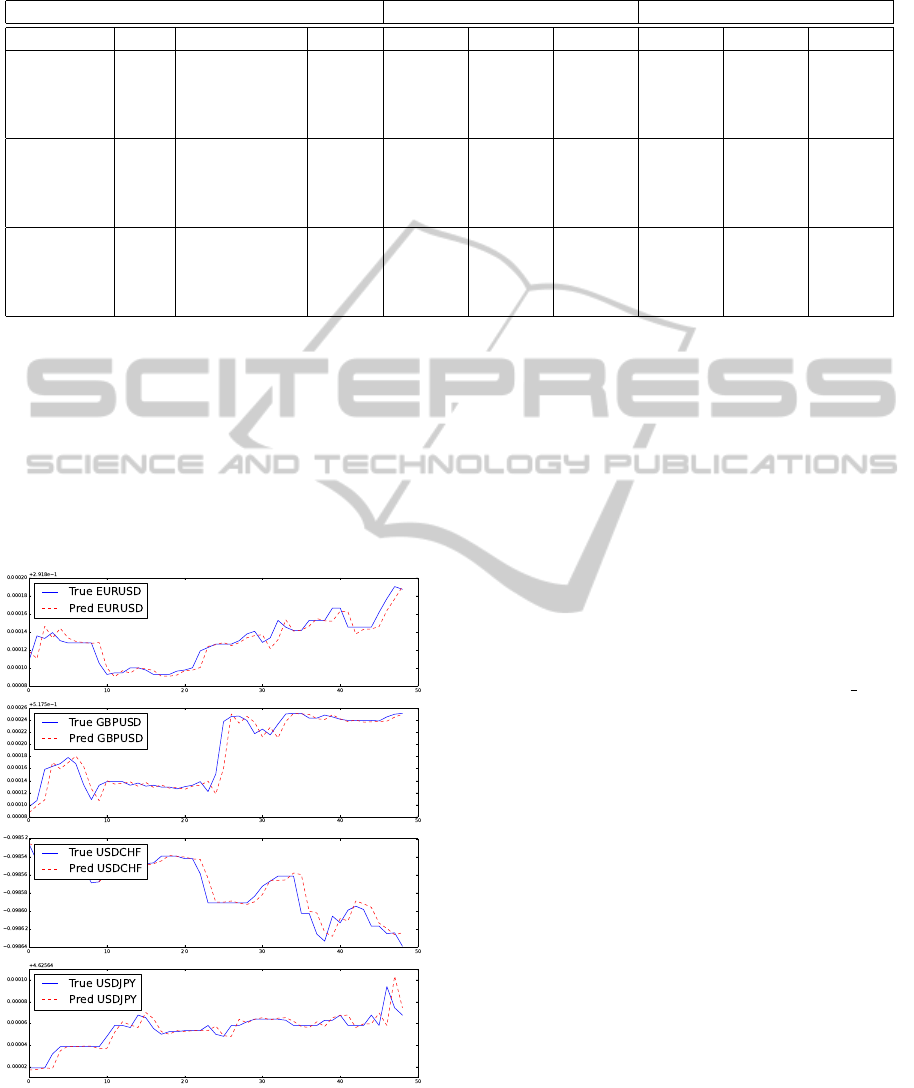
Table 4: Model measures.

Model In-sample Out-of-sample

Method L Parameters e MAPE MAE RMSE MAPE MAE RMSE

OVECM 100 P=2 0.0026 0.00263 0.00085 0.00114 0.00309 0.00094 0.00131

OVECM 400 P=5 0.0041 0.00378 0.00095 0.00127 0.00419 0.00103 0.00143

OVECM 700 P=3 0.0032 0.00323 0.00099 0.00130 0.00322 0.00097 0.00132

OVECM 1000 P=3 0.0022 0.00175 0.00062 0.00087 0.00172 0.00061 0.00090

SLVECM 100 P=2 - 0.00262 0.00085 0.00113 0.00310 0.00095 0.00132

SLVECM 400 P=5 - 0.00375 0.00095 0.00126 0.00419 0.00103 0.00143

SLVECM 700 P=3 - 0.00324 0.00099 0.00130 0.00322 0.00098 0.00132

SLVECM 1000 P=3 - 0.00174 0.00061 0.00087 0.00172 0.00061 0.00090

SLARIMA 100 p=2, d=1, q=1 - 0.00285 0.00110 0.00308 0.00312 0.00098 0.00144

SLARIMA 400 p=1, d=1, q=1 - 0.00377 0.00101 0.00128 0.00418 0.00106 0.00145

SLARIMA 700 p=2, d=1, q=1 - 0.00329 0.00102 0.00136 0.00324 0.00097 0.00133

SLARIMA 1000 p=2, d=1, q=1 - 0.00281 0.00074 0.00105 0.00177 0.00063 0.00092

which models with good in-sample performance are

not necessarily good out-of-sample models. More-

over OVECM outperformed SLARIMA using the

same window size.

Figure 2 shows the out-of-sample forecasts made

by our proposal OVECM with the best parameters

found based on table 4 which follows the time series

very well.

Figure 2: OVECM forecasting accuracy example for 50

minutes using L = 1000 and p = 3.

5 CONCLUSIONS

A new online vector error correction method was pre-

sented. We have shown that our proposed OVECM

considerably reduces execution times without com-

promising solution accuracy. OVECM was compared

with VECM and ARIMA with the same sliding win-

dow sizes and OVECM outperformed both in terms

of execution time. Traditional VECM slightly outper-

formed our proposal but the OVECM execution time

is lower. This reduction of execution time is mainly

because OVECM avoids the cointegration vector cal-

culation using the Johansen method. The condition

for getting new vectors is given by the mean error

variable which controls how many times the Johansen

method is called. Additionally, OVECM introduces

matrix optimization in order to get the new model in

an iterative way. We could see that our algorithm took

much less than a minute at every step. This means that

it could also be used with higher frequency data and

would still provide responses before new data arrives.

For future study, it would be interesting to im-

prove the out-of-sample forecast by considering more

explicative variables, to increase window sizes or try-

ing new conditions to obtain new cointegration vec-

tors.

Since OVECM is an online algorithm which opti-

mizes processing time, it could be used by investors

as an input for strategy robots. Moreover, some tech-

nical analysis methods could be based on its output.

AnOnlineVectorErrorCorrectionModelforExchangeRatesForecasting

199

REFERENCES

Arce, P. and Salinas, L. (2012). Online ridge regression

method using sliding windows. 2011 30th Interna-

tional Conference of the Chilean Computer Science

Society, 0:87–90.

Banerjee, A. (1993). Co-integration, Error Correction,

and the Econometric Analysis of Non-stationary Data.

Advanced texts in econometrics. Oxford University

Press.

Cesa-Bianchi, N., Conconi, A., and Gentile, C. (2005). A

second-order perceptron algorithm. SIAM J. Comput.,

34(3):640–668.

Cesa-Bianchi, N. and Lugosi, G. (2006). Prediction, Learn-

ing, and Games. Cambridge University Press, New

York, NY, USA.

Crammer, K., Dekel, O., Keshet, J., Shalev-Shwartz, S.,

and Singer, Y. (2006). Online passive-aggressive al-

gorithms. Journal of Machine Learning Research,

7:551–585.

Dukascopy (2014). Dukascopy historical data feed.

Duy, T. A. and Thoma, M. A. (1998). Modeling and fore-

casting cointegrated variables: some practical experi-

ence. Journal of Economics and Business, 50(3):291–

307.

Engle, R. F. and Granger, C. W. J. (1987). Co-Integration

and Error Correction: Representation, Estimation, and

Testing. Econometrica, 55(2):251–276.

Engle, R. F. and Patton, A. J. (2004). Impacts of trades in

an error-correction model of quote prices. Journal of

Financial Markets, 7(1):1–25.

Herlemont, D. (2003). Pairs trading, convergence trading,

cointegration. YATS Finances & Techonologies, 5.

Johansen, S. (1988). Statistical analysis of cointegration

vectors. Journal of Economic Dynamics and Control,

12(2-3):231–254.

Johansen, S. (1995). Likelihood-Based Inference in Cointe-

grated Vector Autoregressive Models. Oxford Univer-

sity Press.

Mukherjee, T. K. and Naka, A. (1995). Dynamic re-

lations between macroeconomic variables and the

japanese stock market: an application of a vector er-

ror correction model. Journal of Financial Research,

18(2):223–37.

Rosenblatt, F. (1958). The Perceptron: A probabilistic

model for information storage and organization in the

brain. Psychological Review, 65:386–408.

Vovk, V. (2001). Competitive on-line statistics. Interna-

tional Statistical Review, 69:2001.

Zhang, T. (2004). Solving large scale linear prediction prob-

lems using stochastic gradient descent algorithms. In

ICML 2004: Proceedings of the twenty-ﬁrst inter-

national conference on Machine Learning. OMNI-

PRESS, pages 919–926.

ICPRAM2015-InternationalConferenceonPatternRecognitionApplicationsandMethods

200