A Block-based Approach for Malignancy Detection within the Prostate

Peripheral Zone in T2-weighted MRI

Andrik Rampun

, Paul Malcolm

and Reyer Zwiggelaar

Department of Computer Science, Aberystwyth University, Aberystwyth SY23 3DB, U.K.

Department of Radiology, Norfolk & Norwich University Hospital, Norwich NR4 7UY, U.K.

Keywords:

Prostate Cancer Detection, MRI, Block-based approach, Grey Levels Appearance.

Abstract:

In this paper, a computer-aided diagnosis method is proposed for the detection of prostate cancer within the

peripheral zone. Firstly, the peripheral zone is modelled according to the generic 2D mathematical model from

the literature. In the training phase, we captured 334 samples of malignant blocks from cancerous regions

which were already deﬁned by an expert radiologist. Subsequently, for every unknown block within the

peripheral zone in the testing phase we compare its global, local and attribute similarities with training samples

captured previously. Next we compare the similarity between subregions and ﬁnd which of the subregion has

the highest possibility of being malignant. An unknown block is considered to be malignant if it is similar

in comparison to one of the malignant blocks, its location is within the subregion which has the highest

possibility of being malignant and there is a signiﬁcant difference in lower grey level distributions within the

subregions. The initial evaluation of the proposed method is based on 260 MR images from 40 patients and we

achieved 90% accuracy and sensitivity and 89% speciﬁcity with 5% and 6% false positives and false negatives,

respectively.

1 INTRODUCTION

Prostate cancer is the most commonly diagnosed can-

cer among men and remains the second leading cause

of cancer death in men. In 2013, there were ap-

proximately 240,000 and 40,000 cases reported in

the United States and United Kingdom respectively,

and is estimated to reach 1.7 million cases globally

by 2030 (Howlader et al., 2013; Chou et al., 2010;

PCUK, 2014). In the last decade, prostate cancer

screening has been receiving more attention because

it can help to detect cancer at an early stage before

there are any symptoms. Nowadays, clinical diag-

nostic tools are very popular and globally used de-

spite their inconsistency (60% - 90%) in producing

accurate results (Yu and Hricak, 2000). Many fac-

tors causing this inconsistency such as random biopsy

tests (hence, higher chance of cancerous tissues being

missed), less sensitivity to detect slow-growing and

non-aggressive tumors (as a result tumors often de-

tected in the late age (above 70 years old)), inaccurate

results (e.g. an elevated level of PSA in the blood does

not necessarily indicate cancer), etc.

Computer-aided diagnosis (CAD) of prostate mag-

netic resonance imaging (MRI) has the potential to

improve the results of clinical diagnostic tools. Un-

fortunately, prostate MRI requires a high level of

expertise and suffers from observer variability (Vos

et al., 2010). CAD systems can be of beneﬁt to im-

prove the diagnostic accuracy of clinical methods, re-

duce variability and speed up the reading time of clin-

icians (Vos et al., 2010). In contrast to segmentation

algorithms, detection algorithms only try to decide if

tumor is present and output the approximate tumor

location instead of providing a complete segmenta-

tion. Therefore, the main goal of our research is to

develop CAD methods which automatically delineate

and localise malignant regions, leading to a reduction

of search and interpretation errors, as well as a re-

duction of the variation between and within observers

(Vos et al., 2010). In this paper, we propose a block-

based approach to ﬁnd malignant regions within the

prostate peripheral zone. A block-based approach is

chosen due to its efﬁciency in comparison to a pixel

by pixel sliding window approach (see section 4). The

key idea of this method is, a block or patch is con-

sidered being malignant if its grey levels distribution

is similar with our training samples. We use speciﬁc

metrics to measure similarity for malignancy detec-

tion which will be explained in section 3.3.

Rampun A., Malcolm P. and Zwiggelaar R..

A Block-based Approach for Malignancy Detection within the Prostate Peripheral Zone in T2-weighted MRI.

DOI: 10.5220/0005179000560063

In Proceedings of the International Conference on Bioimaging (BIOIMAGING-2015), pages 56-63

ISBN: 978-989-758-072-7

 2015 SCITEPRESS (Science and Technology Publications, Lda.)

2 PERIPHERAL ZONE MODEL

Pathologically, 80%− 85% of the cancers arise in the

Peripheral Zone (PZ) and the rest are within the cen-

tral zone (Edge et al., 2010). Since the percentage oc-

currence of abnormality in the peripheral zone is high,

we aim to detect prostate abnormality within that re-

gion similar to studies in (Artan and Yetik, 2012), (Ito

et al., 2003) and (Ocak et al., 2007). We did not

perform prostate segmentation because all prostates

were already delineated by our expert radiologist (the

same in (Artan and Yetik, 2012)). To automatically

capture the PZ, we used a generic 2D mathematical

model proposed in (Rampun et al., 2014c; Rampun

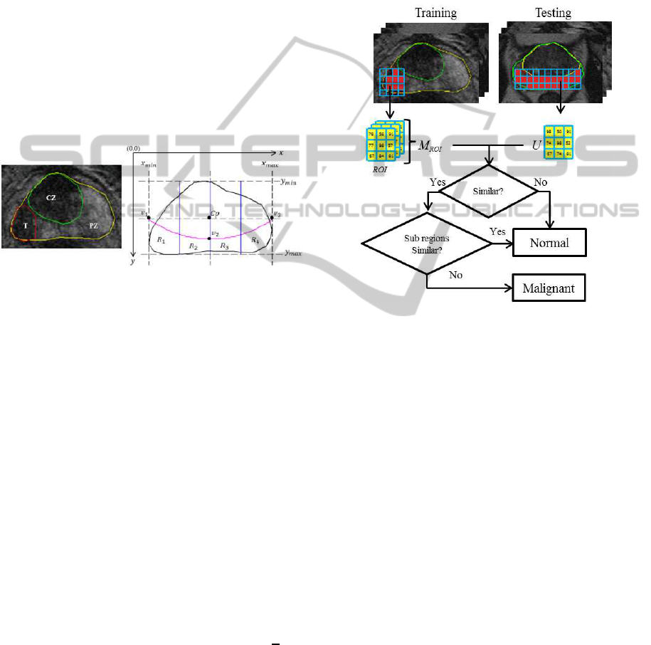
et al., 2013). Figure 1 shows an example of prostate

MRI with its ground truth and the generic 2D prostate

model.

Figure 1: Prostate gland (yellow), peripheral zone (PZ), tu-

mor (T) in red and central zone (CZ) in green. Prostate

gland (black) and the deﬁned PZ boundary y = ax

+bx+c

(magenta) which goes through v

and v

The prostate’s PZ is deﬁned using the quadratic equa-

tion y = ax

+bx+c based on three crucial coordinate

points of the prostate which are v

and v

. They are

determined by the outmost x and y coordinates of the

prostate boundary which are x

min

max

min

max

(see

Figure 1). For example, x

min

and y

max

can be deter-

mined by taking the minimum x and maximum y co-

ordinates along the prostate boundary. Moreover, the

x coordinates of v

and v

are captured from x

min

and

max

and their y coordinate is determined by taking

the y coordinate between y

min

and y

max

. Mathemati-

cally, these can be represented equations (1), (2), (3)

and (4).

= ((x

min

+ x

max

)/2,(y

min

+ y

max

)/2) (1)

= (x

min

,(y

min

+ y

max

)/2) (2)

= ((x

min

+ x

max

)/2,y

min

+ ((y

max

− y

min

) ×

))

(3)

= (x

max

,(y

min

+ y

max

)/2) (4)

where C

is the central coordinate of the prostate

gland. Once the coordinates of v

and v

are

deﬁned, we can determine the boundary of the PZ.

Finally, the PZ region is divided into four subre-

gions (R

, R

and R

) according to the prostate

anatomy in the European consensus guidelines divi-

sion of prostate gland (Dickinson et al., 2011).

3 METHODOLOGY

Figure 2: An overview of the proposed methodology.

Figure 2 shows the summary of the proposed method-

ology. In the training phase, we capture region of in-

terests (ROI, also known as a block) from tumor re-

gions. In Figure 2, M

ROI

contains many collections of

ROIs which basically represents different patterns of

grey level distribution within malignant regions. Sub-

sequently, in the testing phase each unknown block

(U) within the PZ is compared with every block in

ROI

. Based on the comparison results, if U is simi-

lar (measured using speciﬁc metrics) with any blocks

in M

ROI

, then we assume U is most likely being ma-

lignant.

3.1 Preprocessing

Similar to the study in (Artan and Yetik, 2012), each

image MRI is median ﬁltered to reduce noises as well

as to preserve sharp regional boundaries (in our case

we want to preserve the information-bearing struc-

tures such as tumor’s edge boundaries).

3.2 Training

In training phase, we captured 334 number of ma-

lignant blocks (334 of ROIs as illustrated in 2) sized

ABlock-basedApproachforMalignancyDetectionwithintheProstatePeripheralZoneinT2-weightedMRI

7× 7 (this size gives the best quantitative experimen-

tal results, see experimental results) from 5 patients

(50 malignant regions of 50 MRI slices/images). Note

that, each malignant region is already delineated by

an expert radiologist. For every malignant region in

MRI image, we divide it into blocks (ROI) and only

take ROI if all of its elements are within the tumor re-

gion (red in ﬁgure 2). This means ROI is excluded if

one or more of the pixels within the block is outside

the tumor boundary to ensure reliability in our train-

ing samples (we want to make sure that our training

samples are purely taken from malignant tissues). At

the end of this process, M

ROI

contains 334 number of

malignant blocks as shown in equation (5).

ROI

(i) = {ROI

,ROI

....ROI

} (5)

where i is the i

block in M

ROI

3.3 Testing

In the testing phase, for each unknown block (U)

we compare its similarity with every block in M

ROI

(hence there will be 334 comparisons for every U). If

U is similar with one of the blocks in M

ROI

, we as-

sume that the PZ has higher possibility of being ma-

lignant. Note that for block´s size selection, we per-

formed exactly the same in the training phase within

the prostate gland and PZ boundaries. On the other

hand, we used the following metrics to measure sim-

ilarity between U and M

ROI

: global similarity, local

similarity and attribute similarity which have the min-

imum and maximum values of 0 and 1.0, respectively.

In all cases we use a default threshold 0.5 which

means if the similarity is more than half of its max-

imum similarity value (1.0), U is considered being

malignant. According to (Ali et al., 2005) the human

eye is less sensitive in perceiving a change in shape

and texture if the similarity percentage between two

objects is less than 50% (hence studies in (Ali et al.,

2005; Hasan et al., 2009; Hasan et al., 2012) have

used a default threshold 0.5 in measuring similarity

between two textures). In fact, a study conducted

by (Chen et al., 2006) discussed the use of decision

threshold (minimum and maximum are 0 and 1, re-

spectively) adjustment in classiﬁcation for cancer pre-

diction concluded that when the sample sizes are sim-

ilar (in our case each U and ROI are the same size),

they suggested that the optimal decision threshold and

balanced decision is approximately 0.5 as their exper-

imental results show high concordance with a balance

between sensitivity and speciﬁcity. When estimating

string similarity, (Elita et al., 2007) considers the se-

quence of common elements have to be at least 50%

in both strings to be considered similar.

3.3.1 Global Similarity

Global similarity (G) measures the number of ele-

ments (#U) in U within the range of i

block in

ROI

. This metric does not concern about the indi-

vidual grey level value in ROI

but the overall range.

To calculate the global similarity:

1. Calculate the mean (ROI

mean

) and standard devia-

tion (ROI

std

)

2. Calculate its lower (ROI

Lrange

) and upper

(ROI

Urange

) ranges using equation (6) and (7)

3. Calculate G using equation (8)

ROI

Lrange

= ROI

mean

− ROI

std

(6)

ROI

Urange

= ROI

mean

+ ROI

std

(7)

ROI

Lrange

≤ #U ≤ ROI

Urange

n× m

(8)

where n and m are the size of the block. Equation (8)

calculates similarity based on the number of elements

inU within the range of i

block in M

ROI

. This means

the more elements in U within the range of i

block,

the more similar they are (leads to higher possibility

being malignant).

3.3.2 Local Similarity

Local similarity (L) measures the amount of overlap-

ping information between two blocks. In comparison

to global similarity, this metric compares correspond-

ing elements in U and ROI

. For every U we measure

its L using equation (9).

∑

min{U(z),ROI

(z)}

∑

max{U(z),ROI

(z)}

(9)

where z represents every single element in a block. In

this measure, the higher the overlapping value means

the more similar the blocks (between U and ROI

3.3.3 Attribute Similarity

Attribute similarity (A) measures the number of oc-

currences of unique overlapping grey levels between

two blocks. This means only grey levels appear in

both blocks will be taking into account. This metric

can be calculated using the following steps:

1. Find unique elements in U and ROI

, let say

unique

and ROI

unique

2. Count the number of grey level occurrences in

unique

and ROI

unique

, let say f

unique

and f

ROI

unique

3. Find the overlapping elements in U

unique

and

ROI

unique

, let say U

unique

∩ ROI

unique

BIOIMAGING2015-InternationalConferenceonBioimaging

4. Count the number of occurrences for ev-

ery element in U

unique

and ROI

unique

, let say

unique

∩ROI

unique

5. Use equation (10) to calculate A

∑

unique

∩ROI

unique

∑

unique

∪ROI

unique

(10)

where f

unique

∪ROI

unique

represents the number of grey

levels occurrences in both U and ROI

(the same as

the number of grey levels in U and ROI

3.4 Subregion Similarity

In addition to the metrics in section 3.3, we use his-

togram intersection distance (d) to measure the simi-

larity between two subregions’ histograms (e.g. his-

togram from R

and R

in Figure 1) by measuring

their distance in the intersection space (Rubner et al.,

2000). Previous studies (Rampun et al., 2014b; Ram-

pun et al., 2014a) have shown that the peripheral

zone has higher chance of being malignant if one

of the subregions contains a signiﬁcant number of

lower grey levels (e.g. below 120) in comparison

to the other subregions. For example, R

contains

80% lower grey levels whereas R

, R

and R

are

dominated by upper grey levels (this makes R

looks

darker in T2-Weighted-MRI image in comparison to

the other subregions). Several studies suggested that

prostate cancer tissue tends to appear darker on T2-

weighted MRI images (Garnick et al., 2012; Ginat

et al., 2009; Taneja, 2004; Mohamed et al., 2003).

Moreover, radiologists also tend to use regions in-

tensity (e.g. darker region is more likely to be ma-

lignant) to identify abnormality within the peripheral

zone (Edge et al., 2010). Therefore, the main ob-

jective of this metric is to ﬁnd subregion which has

the highest possibility of being malignant. We chose

this metric because of its capability to handle partial

matches when the areas of two regions are different

(Rubner et al., 2000). In our case, every area of sub re-

gion is different (due to PZ and prostate boundaries).

For each subregion (e.g. R

), we contsruct grey level

histogram (255 bins) by assigning every pixel to its

appropriate grey level and normalise it to sum equal to

1. After normalisation, we calculate the histogram’s

mean value to roughly identify which subregion has

the highest number of lower grey levels. The same

process applied to the other subregions (R

, R

and

). Subsequently, we take histograms with the low-

est and highest histogram mean values and calculate

d using equation (11).

d = 1 − (

∑

j=1

min{H

max

( j),H

min

( j)}/

∑

j=1

max

( j))

(11)

where j represents each bin in the histogram and H

max

and H

min

are subregions’ histograms which have the

highest and lowest histogram mean values, respec-

tively. In contrast to the metrics in section 3.3, smaller

d indicates higher similarity as it means smaller dis-

tance separates two histograms in the intersection dis-

tance (hence lower possibility of the PZ being malig-

nant).

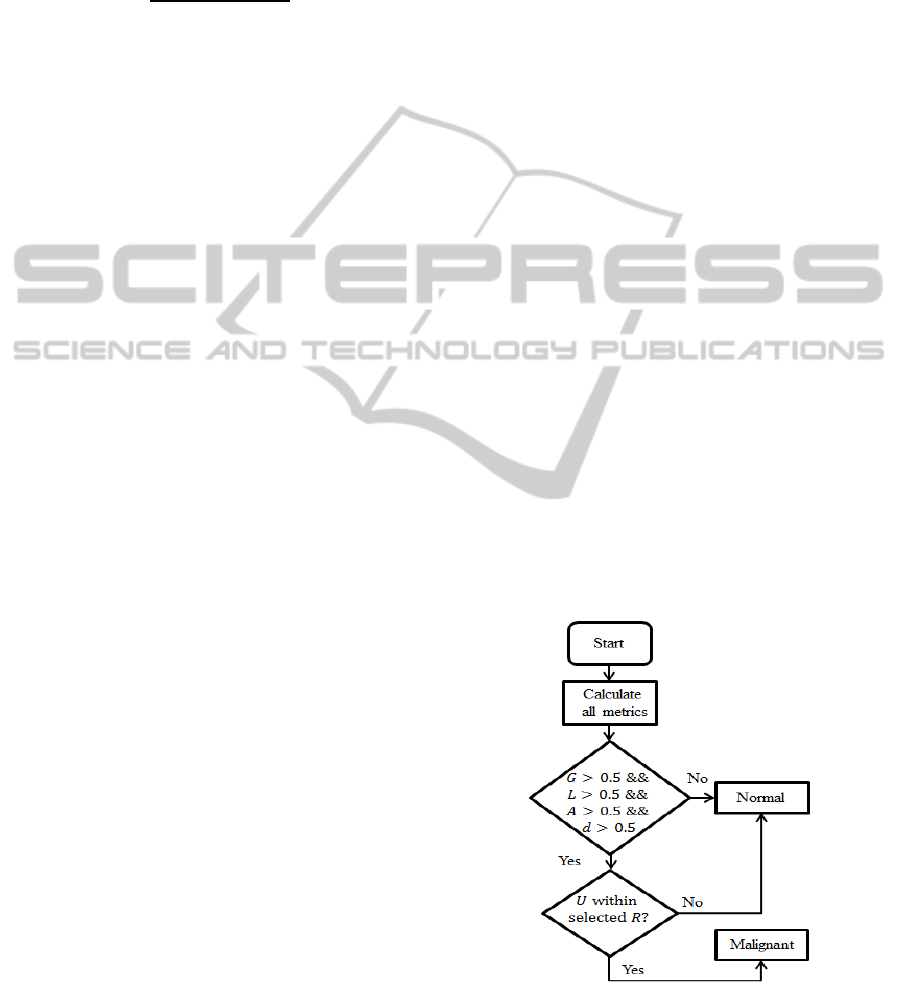
3.5 Malignancy Detection

An unknown sample/block (U) is considered to be

malignant if all of the following conditions are true:

1. If its G, L and A are greater than 0.5 and

2. If d > 0.5 and

3. If the location of U is within the subregion with

the lowest histogram mean value

Figure 3 shows the ﬂow chart decision rules for ma-

lignancy detection in the proposed method. Note that

the selected R is the subregion with the lowest his-

togram mean value. If the location of the segmented

region is not within the subregion which has the low-

est histogram mean value, we do not consider U as

malignant because previous studies (Rampun et al.,

2014b; Rampun et al., 2014a) shows that in many

cases cancerous region has lower intensity as previ-

ously mentioned in (Garnick et al., 2012; Ginat et al.,

2009; Taneja, 2004; Mohamed et al., 2003). Note that

Figure 3: Flow chart decision rule.

the threshold 0.5 is selected based on the studies con-

ducted by (Chen et al., 2006; Ali et al., 2005; Hasan

et al., 2009; Hasan et al., 2012; Elita et al., 2007) in

ABlock-basedApproachforMalignancyDetectionwithintheProstatePeripheralZoneinT2-weightedMRI

different applications. Hence, we did not perform ex-

periments to determine a new threshold value due to

the extensive experiments have been done in the liter-

ature.

4 EXPERIMENTAL RESULTS

For evaluation, our database contains 260 MRI im-

ages (118 images are identiﬁed as malignant and 142

are benign/normal) from 40 different patients aged 54

to 74 collected from the Norfolk and Norwich Univer-

sity Hospital. The prostates, cancers and central zones

were delineated by an expert radiologist on each of

the MRI images and all malignant lesions are biopsy

proven. Each image was analysed and classiﬁed as

to whether the prostate contains malignancy (and seg-

ment the approximate tumor location) based on the

decision rules explained in section 3.5. Subsequently,

we compared the result with the ground truth whether

the prostate contains malignancy or not. The pro-

posed method achieved 90% accuracy and sensitivity

and 89% speciﬁcity with 5% and 6% false positives

and false negatives, respectively. Note that the term

accuracy here means correct classiﬁcation rate (CCR)

which means if an image is classiﬁed as containing

malignancy and the ground truth is malignant then the

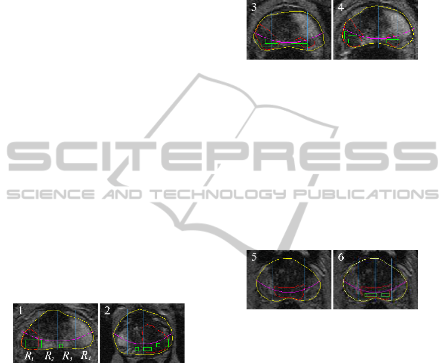
image is classiﬁed correctly. The ﬁrst two examples

in Figure 4 shows the results of two MR images con-

taining malignant region in each of them.

Figure 4: Examples of malignant cases.

The ground truth of malignant regions are within the

red lines and green blocks are blocks identiﬁed as ma-

lignant. For every case, we use a generic PZ mathe-

matical model in section 2 to deﬁne the PZ bound-

ary (magenta line) and divide the PZ model into four

subregions (partitioned by the blue lines). As we can

see in image 1 and 2 the segmented blocks are within

the malignant regions indicating correct classiﬁcation

and approximate location. In image 1, a small block

segmented within R

(false positive) which indicates

malignancy. However, since the subregion R

has the

lowest average grey level value (and d > 0.5), we con-

sider the segmented region in R

has higher possibil-

ity of being malignant and only consider blocks in R

Similarly in image 2, segmented blocks in R

are con-

sidered having higher possibility of being malignant

because subregion R

has the lowest grey level aver-

age value (and d > 0.5), hence a segmented block in

are considered to have lower possibility of being

malignant.

Figure 5: Examples of cases with two malignant regions.

Figure 5 shows examples of MR images containing

two malignant regions. In both image 3 and 4, sub-

region R

has the lowest grey level mean value and

d > 0.5. The results show that most malignant blocks

were found to be malignant within the cancerous re-

gions (red lines). We also can see some segmented

blocks within the second malignant regions in both

images. On the other hand, Figure 6 shows examples

of segmentation results using different window sizes.

In image 5, there is no segmented region using 9 × 9

window size but we can clearly see several regions

were segmented in image 6 using 7× 7 window. This

indicates bigger window size decreases the sensitivity

rate and increases the speciﬁcity rate.

Figure 6: Examples of segmentation results using different

window sizes.

We tested the accuracy, sensitivity and speciﬁcity of

the proposed method using different window sizes of

3× 3, 5× 5, 7 × 7, 9× 9 and 11× 11. Based on the

results shown in Figure 7, sensitivity increases using

a small size of window 3× 3 and gradually decreases

as the window size is getting bigger. On the other

hand, speciﬁcity decreases using a small window and

increases when a bigger window size is used (e.g.

9× 9). A balanced results in terms of accuracy, sen-

sitivity and speciﬁcity were achieved using a medium

window size of 7× 7.

Various methods using different frameworks, modali-

ties and features have been proposed in the literature

and our method achieved similar results. Neverthe-

less, it is extremely difﬁcult to make a quantitative

comparison due to the differences in datasets (differ-

ent modalities such as T2-weighted MRI, diffusion-

weighted MRI, etc) and frameworks (e.g. combining

different modalities) used in the other studies. In fact,

absence of public datasets also makes a quantitative

BIOIMAGING2015-InternationalConferenceonBioimaging

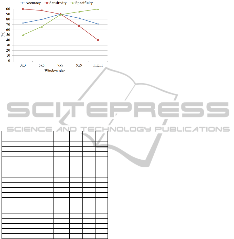
Figure 7: Accuracy, sensitivity and speciﬁcity using differ-

ent window sizes.

comparison of methodologies in the literature is im-

possible. However, to have an overall qualitative es-

timate of the functioning of our method we compared

with some of the previous studies in Table 1.

Table 1: Results are ordered based on accuracy, sensitivity

and speciﬁcity, respectively (all measured in %).

Authors Cases Acc Sen Spe

Our method 40 90 90 89

(Sung et al., 2011) 42 89 89 89

(Vos et al., 2010) 29 89 - -

(Ampeliotis et al., 2007) 10 87 - -

(Tiwari et al., 2010) 19 84 - -

(Rampun et al., 2014c) 25 82 81 84

(Artan and Yetik, 2012) 15 82 76 86

(Tabesh et al., 2007) 29 81 - -

(Kim et al., 2006) 20 75 73 77

(Han et al., 2008) 46 - 96 92

(Engelbrecht et al., 2003) 36 - 93 -

(Shimofusa et al., 2005) 60 - 93 -

(Ito et al., 2003) 111 - 87 74

(Litjens et al., 2011) 188 - 83 -

(Niaf et al., 2012) 30 - 82 -

(Futterer et al., 2006) 6 - 83 83

(Miao et al., 2007) 30 - 76 70

(Ocak et al., 2007) 50 - 73 88

(Llobet et al., 2007) 303 - 57 61

(Schlemmer et al., 2004) 28 - - 68

From the qualitative comparisons in Table 1, the pro-

posed method achieved similar results with the state

of the arts in all metrics (accuracy, sensitivity and

speciﬁcity). Note that some of the authors did not

report one or two of their results. In terms of ac-

curacy and sensitivity, our method achieved the best

result in comparison to the other methods in Table

1. However, the proposed method of (Sung et al.,

2011) achieved similar results in all metrics of 89%.

(Vos et al., 2010) and (Ampeliotis et al., 2007) did

not report sensitivity and speciﬁcity of but their pro-

posed methods achieved similar results 89% and 87%,

respectively. For sensitivity, (Han et al., 2008) re-

ported their proposed method achieved 96% which is

the highest in Table 1 where the proposed methods of

(Engelbrecht et al., 2003) and (Shimofusa et al., 2005)

achieved 93% followed by our method 90%. (Llobet

et al., 2007) achieved 57% sensitivity based on 303

number of cases where (Litjens et al., 2011) achieved

83% in 188 number of cases. Finally, in terms of

speciﬁcity, the proposed method of (Han et al., 2008),

once again achieved the highest result of 92% where

our proposed method achieved 89% similar with the

methods proposed by (Sung et al., 2011), and (Ar-

tan and Yetik, 2012). (Llobet et al., 2007) once again

achieved the lowest result of 61% but evaluated based

on the largest dataset in Table 1.

These comparisons are subjective as results are highly

inﬂuenced by the number of datasets, different modal-

ities and methods frameworks. For example although

the method proposed of (Llobet et al., 2007) produced

the lowest sensitivity and speciﬁcity but the evalua-

tion is based on 303 prostates. On the other hand, al-

though (Han et al., 2008) achieved the highest sensi-

tivity and speciﬁcity (based on Table 1 ) but was eval-

uated with smaller dataset contains 46 ultrasound im-

ages (46 patients). Similarly, although the proposed

method achieved 90% for both accuracy and sensitiv-

ity, these are based on a speciﬁc window size (7× 7).

The performance of the proposed method vary ac-

cording to window sizes (e.g accuracy 72% and 80%

with 3 × 3 and 5 × 5 window size, respectively, see

7). In terms of computationally complexity, the pro-

posed method took approximately 3 hours 30 minutes

in both training and testing phases (310 MRI images,

Matlab 2013, Windows 7 Intel core i5). On the other

hand using a pixel by pixel sliding window approach

took approximately 30 hours for the entire experiment

with 7× 7 window size. Using smaller window size

(e.g. 5× 5) took even longer. Therefore we chose

block based approach due to its speed performance.

5 DISCUSSIONS

In contrast to the earlier methods, our method is dif-

ferent in the sense that:

1. We only used a single modality for abnormal-

ity detection which is T2-Weighted MRI whereas

(Engelbrecht et al., 2003) used multimodality

such as diffusion MRI and MR Spectroscopy.

2. The method in (Han et al., 2008) used additional

clinical knowledge (e.g. shape of the region) to

discriminate cancer regions in addition of image

features while our method only used the informa-

tion of grey level distributions between two sam-

ples to achieve similar results.

ABlock-basedApproachforMalignancyDetectionwithintheProstatePeripheralZoneinT2-weightedMRI

3. The methods in (Ocak et al., 2007; Sung et al.,

2011) used various perfusion parameters on a sin-

gle modality while our method is purely based

on the information of grey level distributions to

achieve similar results.

This paper makes three contributions:

1. A novel approach of CAD diagnosis method

which is based on similarity measure between un-

known and sample blocks.

2. The development of the proposed method and its

application in prostate cancer detection and local-

isation using a single MRI modality with compa-

rable results to the state-of-the-art methods in the

literature.

3. We introduced a simple approach in measuring

similarity based on the occurrences of overlapping

grey levels between two samples (section 3.3.3).

6 CONCLUSIONS

The proposed method could help clinicians to perform

targeted biopsies which ought to be better and poten-

tially improve the accuracy of prostate cancer diagno-

sis. In conclusion, we have presented a novel method

of prostate cancer detection and localisation within

the PZ. In this paper we have showed the potential

of grey level information (G, L and A) in predicting

malignancy by comparing each unknownsample with

malignant samples. In addition to that, we also have

used statistical grey levels information (mean value)

to ﬁnd subregion which has the most possibility of be-

ing malignant. By combining these information, we

achieved promising and similar results with the state

of the arts in the literature. Nevertheless, the best

results were achieved using 7 × 7 window size and

achieved lower accuracy and speciﬁcity in smaller

window sizes.

REFERENCES

Ali, M. A., Dooley, L. S., and Karmakar, G. C. (2005). Au-

tomatic feature set selection for merging image seg-

mentation results using fuzzy clustering. In Inter-

national Conference on Computer and Information

Technology.

Ampeliotis, D., Antonakoudi, A., Berberidis, K., and

Psarakis, E. Z. (2007). Computer aided detection of

prostate cancer using fused information from dynamic

contrast enchanced and morphological magnetic res-

onance images. In IEEE International Conference

on Signal Processing and Communications(ICSPC

2007). IEEE Xplore.

Artan, Y. and Yetik, I. S. (2012). The digital rectal exami-

nation (dre) remains important outcomes from a con-

temporary cohort of men undergoing an initial 12-18

core prostate needle biopsy. Can J Urol, 16(6):1313

–1323.

Chen, J. J., Tsai, C., Moon, H., Ahn, H., Young, J. J., ,

and Chen, C. (2006). The use of decision threshold

adjustment in classiﬁcation for cancer prediction.

http://www.ams.sunysb.edu/∼hahn/psﬁle/papthres.pdf.

Accessed 19-June-2014.

Chou, R., Croswell, J. M., Dana, T., Bougatsos, C., Blaz-

ina, I., Fu, R., Gleitsmann, K., Koenig, H. C., Lam,

C., Maltz, A., Rugge, J. B., and Lin, K. (2010). A

review of the evidence for the u.s. preventive services

task force. http://www.uspreventiveservicestaskforce.

org/uspstf1 2/prostate/prostateart.htm/. Accessed 15-

November-2013.

Dickinson, L., Ahmed, H. U., Allen, C., Barentsz, J. O.,

Carey, B., Futterer, J. J., Heijmink, S. W., Hoskin,

P. J., Kirkham, A., Padhani, A. R., Persad, R., Puech,

P., Punwani, S., Sohaib, A. S., Tombal, B., Villersm,

A., v. der Meulen, J., and Emberton, M. (2011). Mag-

netic resonance imaging for the detection, localisa-

tion, and characterisation of prostate cancer: recom-

mendations from a european consensus meeting. Eur

Urol, 59(4):477–494.

Edge, S. B., Byrd, D. R., Compton, C., Fritz, A. G., Greene,

F. L., and Trotti, A. (2010). AJCC Cancer Staging

Manual. Springer, Chicago, 7th edition.

Elita, N., Gavrila, M., and Cristina, V. (2007). Experiments

with string similarity measures in the ebmt frame-

work. In Proceedings of the RANLP 2007 Conference.

Engelbrecht, M. R., Huisman, H. J., Laheij, R. J., Jager,

G. J., van Leenders, G. J., Kaa, C. A. H.-V. D., de la

Rosette, J. J., Blickman, J. G., and Barentsz, J. O.

(2003). Discrimination of prostate cancer from nor-

mal peripheral zone and central gland tissue by using

dynamic contrast-enhanced mr imaging. Radiology,

229:248–254.

Futterer, J. J., Heijmink, S. W. T. P. J., Scheenen, T. W. J.,

Veltman, J., Huisman, H. J., Vos, P., de Kaa, C.

A. H., Witjes, J. A., Krabbe, P. F. M., Heerschap,

A., and Barentsz, J. O. (2006). Prostate cancer lo-

calization with dynamic contrast-enhanced mr imag-

ing and proton mr spectroscopic imaging. Radiology,

241(2):449–458.

Garnick, M. B., MacDonald, A., Glass, R., and Leighton,

S. (2012). Harvard Medical School 2012: Annual Re-

port on Prostate Diseases. Harvard Medical School.

Ginat, D. T., Destounis, S. V., Barr, R. G., Castaneda, B.,

Strang, J. G., and Rubens, D. J. (2009). Us elastog-

raphy of breast and prostate lesions. Radiographics,

29(7):2007–2016.

Han, S., Lee, H., and Choi, J. (2008). Computer-aided

prostate cancer detection using texture features and

clinical features in ultrasound image. J. Digital Imag,

21(1):121–133.

Hasan, M. M., Ali, M. A., Kabir, M. H., and Sorwar, G.

(2009). Object segmentation using block based pat-

terns. In TENCON 2009 -2009 IEEE Region 10 Con-

ference, pages 1–6.

BIOIMAGING2015-InternationalConferenceonBioimaging

Hasan, M. M., Sharmeen, S., Rahman, M. A., Ali, M. A.,

and Kabir, M. H. (2012). Block based image segmen-

tation. Advances in Communication, Network, and

Computing, 108:15–24.

Howlader, N., Noone, A. M., Krapcho, M., Garshell, J.,

Neyman, N., Altekruse, S., Kosary, C., Yu, M., Ruhl,

J., Tatalovich, Z., Cho, A., Mariotto, H., Lewis, D.,

Chen, H., Feuer, E., and Cronin, K. (2013). Seer can-

cer statistics review,1975-2010, national cancer insti-

tute. http://seer.cancer.gov/csr/1975 2010/. Accessed

16-October-2013.

Ito, H., Kamoi, K., Yokoyama, K., Yamada, K., and

Nishimura, T. (2003). Visualization of prostate can-

cer using dynamic contrast-enhanced mri: compari-

son with transrectal power doppler ultrasound. British

Journal of Radiology, 76(909):617–624.

Kim, K. C., Park, B. K., and Kim., B. (2006). Localiza-

tion of prostate cancer using 3t mri: comparison of

t2-weighted and dynamic contrast-enhanced imaging.

J Comput Assist Tomogr, 30:7–11.

Litjens, G. J. S., Vos, P. C., Barentsz, J. O., Karssemeijer,

N., and Huisman, H. J. (2011). Automatic computer

aided detection of abnormalities in multi-parametric

prostate mri. In Proc.SPIE 7963, Medical Imaging

2011: Computer-Aided Diagnosis. SPIE.

Llobet, R., Juan, C., Cortes, P., Juan, A., and Toselli, A.

(2007). computer-aided detection of prostate can-

cer. International Journal of Medical Informatics,

76(7):547–556.

Miao, H., Fukatsu, H., and Ishigaki, T. (2007). Prostate

cancer detection with 3-t mri: comparison of diffu-

sionweighted and t2-weighted imaging. Eur J Radiol,

61:297–302.

Mohamed, S., El-Saadany, E. F., Abdel-Galil, T., Shen, J.,

Salama, M. M. A., Fenster, A., Downey, D. B., and

Rizkalla, K. (2003). Region of interest identiﬁcation

in prostate trus images based on gabor ﬁlter. In IEEE

46th Midwest Symposium on Circuits and Systems,

volume 1, pages 415–419.

Niaf, E., Rouviere, O., Mege-Lechevallier, F., Bratan, F.,

and Lartizien, C. (2012). Computer-aided diagnosis

of prostate cancer in the peripheral zone using multi-

parametric mri. Phys Med Biol, 57:3833–3851.

Ocak, I., Bernardo, M., Metzger, G., Barrett, T., Pinto, P.,

Albert, P. S., and Choyke, P. L. (2007). Dynamic

contrast-enhanced mri of prostate cancer at 3 t: a study

of pharmacokinetic parameters. American Journal of

Roentgenology, 189(4):W192–W201.

PCUK (2014). Prostate cancer key facts.

http://www.cancerresearchuk.org/cancer-

info/spotcancerearly. Accessed 15-April-2014.

Rampun, A., Malcolm, P., and Zwiggelaar, R. (2013). De-

tection and localisation of prostate abnormalities. In

3rd Computational and Mathematical Biomedical En-

gineering (CMBE’13), pages 204–208.

Rampun, A., Malcolm, P., and Zwiggelaar, R. (2014a).

Computer aided diagnosis method for mri-guided

prostate biopsy within the peripheral zone using grey

level histograms. In 7th International Conference on

Machine Vision (ICMV’14).

Rampun, A., Malcolm, P., and Zwiggelaar, R. (2014b).

Detection and localisation of prostate cancer within

the peripheral zone using scoring algorithm. In 16th

Irish Machine Vision and Image Processing Confer-

ence (IMVIP’14).

Rampun, A., Malcolm, P., and Zwiggelaar, R. (2014c).

Detection of prostate abnormality within the periph-

eral zone using local peak information. In 3rd Inter-

national Conference on Pattern Recognition Applica-

tions and Methods (ICPRAM’14). SCITEPRESS.

Rubner, Y., Tomasi, C., and Guibas., L. J. (2000). The earth

movers distance as a metric for image retrieval. Inter-

national Journal of Computer Vision, 40(2):99–121.

Schlemmer, H. P., Merkle, J., and Grobholz, R. (2004). Can

preoperative contrast-enhanced dynamic mr imaging

for prostate cancer predict microvessel density in

prostatectomy specimens? Eur Radiol, 14:309–317.

Shimofusa, R., Fujimoto, H., Akamata, H., Motoori, K., Ya-

mamoto, S., Ueda, T., and Ito, H. (2005). Diffusion-

weighted imaging of prostate cancer. J Comput Assist

Tomogr, 29:149–153.

Sung, Y. S., Kwon, H.-J., Park, B. W., Cho, G., Lee,

C. K., Cho, K.-S., and Kim, J. K. (2011). Prostate

cancer detection on dynamic contrast-enhanced mri:

Computer-aided diagnosis versus single perfusion pa-

rameter maps. American Journal of Roentgenology,

197(5):1122–1129.

Tabesh, A., Teverovskiy, M., Pang, H. Y., Kumar, V. P.,

Verbel, D., Kotsianti, A., and Saidi, O. (2007). Mul-

tifeature prostate cancer diagnosis and gleason grad-

ing of histological images. IEEE Trans. Med. Imag.,

26(10):1366–1378.

Taneja, S. S. (2004). Imaging in the diagnosis and man-

agement of prostate cancer. Reviews in Urology,

6(3):101–113.

Tiwari, P., Kurhanewicz, J., Rosen, M., and Madabhushi, A.

(2010). Semi supervised multi kernel (sesmik) graph

embedding: identifying aggressive prostate cancer via

magnetic resonance imaging and spectroscopy. In

Medical Image Computing and Computer-Assisted In-

tervention MICCAI. Springer.

Vos, P. C., Hambrock, T., Barentsz, J., and Huisman, H.

(2010). Computer-assisted analysis of peripheral zone

prostate lesions using t2-weighted and dynamic con-

trast enhanced t1-weighted mri. Physics in Medicine

and Biology, 55:1719–1734.

Yu, K. K. and Hricak, H. (2000). Imaging prostate cancer.

Radiol Clin North Am, 38(1):59–85.

ABlock-basedApproachforMalignancyDetectionwithintheProstatePeripheralZoneinT2-weightedMRI