
Empirical Bayesian Models of L1/L2 Mixed-norm Constraints
Deirel Paz-Linares, Mayrim Vega-Hernández and Eduardo Martínez-Montes
Neuroinformatics Department, Cuban Neuroscience Center, Havana, Cuba
1 OBJECTIVES
Inverse problems are common in neuroscience and
neurotechnology, where usually a small amount of
data is available with respect to the large number of
parameters needed for modelling the brain activity.
Classical examples are the EEG/MEG source
localization and the estimation of effective brain
connectivity. Many kinds of constraints or prior
information have been proposed to regularize these
inverse problems. Combination of smoothness (L2
norm-based penalties) and sparseness (L1 norm-
based penalties) seem to be a promising approach
due to its flexibility, but the estimation of optimal
weights for balancing these constraints became a
critical issue (Vega-Hernández et al., 2008). Two
important examples of constraints that combine
L
1
/L
2
norms are the Elastic Net (Vega-Hernández et
al., 2008) and the Mixed-Norm L
12
(MxN, Gramfort
et al., 2012). The latter imposes the properties along
different dimensions of a matrix inverse problem. In
this work, we formulate an empirical Bayesian
model based on an MxN prior distribution. The
objective is to pursue sparse learning along the first
dimension (along rows) preserving smoothness in
the second dimension (along columns), by
estimating both parameter and hyperparameters
(regularization weights).
2 METHODS
The matrix linear Inverse Problem consists in
inferring an SxT parameter matrix in the model
, where (data), (noise) are NxT, is
NxS, with N<<S, making it an ill-posed problem due
to its non-uniqueness. One approach to address this
problem is the Tikhonov regularization which uses a
penalty function
to find the inverse solution
through a penalized least-squares (PLS) regression
‖
‖
, where is the
regularization parameter. Another approach is the
Bayesian theory, where the solution maximizes the
posterior probability density function (pdf), given by
the Bayes equation:
,,
|
∝
|
,
|
,
which is largely equivalent to the PLS model if we
set the likelihood of the data to
|
,
2
|
|
, and the prior
distribution of the parameters as an exponential
function
|
⁄
, where Z is a
normalizing constant.
The first approach has led to development of fast
and efficient algorithms for a wide range of solvers
, but is determined heuristically using
information criteria which often do not provide
optimal values. On the other hand, Bayesian
approach allows inference on the hyperparameters
and
but frequently involving numerical Monte
Carlo calculations that makes it very slow and
computationally intensive. However, recent
developments of approximate models such as
Variational and Empirical Bayes, allow for fast
computation of complex models.
In this work, we propose to use the squared Mixed-
Norm penalty for the parameters, which is defined as
the L
2
norm of the vector obtained from the L
1
norms of all columns
of (Gramfort et al.,
2012) and can be written as
‖
‖
;,
∑‖
‖
,
where is the weights (positive)
diagonal matrix. The prior pdf for this penalty
represents a Markov Random Field (MRF) where
the states of the variable
are not separable.
|
∝
|
||
|
(1)
Using Empirical Bayes, we first transform this MRF
into a Bayesian network, to arrive to a hierarchical
model (figure 1) by reformulating the pdf of each
as
,
, where
. In this way, the
information received by
from
is contained in
an auxiliary magnitude
∑
|
|
, leading to
a Normal-Laplace joint pdf:
,
|
2
|
|
∝
‖
⁄
‖
⁄
;
x
(2)
Then, using the scaled mixture of Gaussians for the
Normal-Laplace pdf (Li and Lin 2010), a hyper-
Paz-Linares D., Vega-Hernández M. and Martínez Montes E..
Empirical Bayesian Models of L1/L2 Mixed-norm Constraints.
Copyright
c
2014 SCITEPRESS (Science and Technology Publications, Lda.)
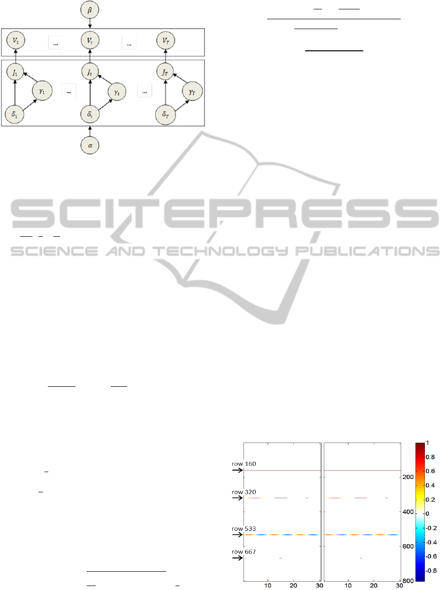
Figure 1: Hierarchical diagram of the Bayesian network
obtained for the mixed-norm L
12
model.
parameter
is introduced to complete the joint
prior
,
,
|
|
,
|
,
|
where the variance matrix for
is diagonal
and the pdf for
is the truncated
Gamma
|
,
1/2,1,
,∞. T
he vector
can be updated from the
estimated in the
previous iteration. Then we can choose gamma non-
informative priors
and
and rewrite the
joint posterior pdf as:
,
,,
|
∝
|
,
,
|
(3)
The maximum a posteriori estimate for the model
parameters
is easily derived from the Gaussian pdf
,
,,
∝
,
,
=
/
,
, with posterior mean and variance:
;
(4)
The estimates for the hyperparameters are achieved
by maximizing the evidence (evidence procedure),
also known as the type II likelihood
L
, which is
obtained by integrating out the parameters
from
the joint posterior pdf in (3).
L
∑
ln
|
|
ln
,,
(5)
with
.
Closed estimates maximizing
L
cannot be obtained due to the nonlinear form of
but it can be rearranged in terms of
,
and other
differentiable expressions of
,,
, which
after
differentiation leads to the following updates for the
hyperparameters:
;
1
16
1
4
(6)
∑∑
2
1
2
∑∑
2
∑‖
|
|‖
∑‖
‖
∑∑
Λ
⁄
(6)
where
/
is related with the
normalizing constant for the TG. Similar to the
Relevance Vector Machine (Tipping 2001), the
hyperparameter
controls the sparseness of the
solution, since it cannot take values equal or below
, allowing the
where this conditions holds to
be set to zero. The iterative estimation of parameters
and hyperparameters with these formulae (4 and 6)
is equivalent to an EM algorithm. Here we illustrate
how this model works with this algorithm (using in-
house code) but future studies will focus in deriving
faster and more efficient algorithms for estimating
the model.
3 RESULTS
Simulations of a matrix (800x30) with different
waveforms (along columns) in well-localized rows,
were performed to test the ability of the model to
estimate simultaneously different levels of
sparseness and smoothness in both dimensions
(figure 2, left). The inverse solution was obtained
(figure 2, right) from data generated using a random
design matrix (100x800,
~N(0,4), SNR=30db),
converging after 150 iterations (in about 5 min).
Estimation of relevant rows is shown in figure 3.
We also considered a more realistic simulation of
the EEG inverse problem. A ring of 736 cortical
generators (voxels defined in MNI brain atlas), was
used to simulate 3 spatio-temporal sources. The
electric lead field was computed as the
Figure 2: Left: Simulated matrix. Right: Estimated with
the Bayesian MxN model, using an EM algorithm.
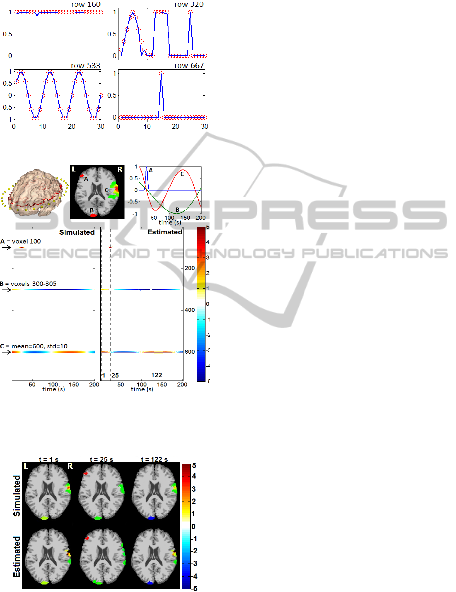
Figure 3: Simulated (true, red circles) and estimated (blue
line) inverse solution for rows arrowed in figure 2.
Figure 4: Realistic simulation (ring of cortical generators).
Parameter matrix was formed by simulated sources A (1
voxel, temporal bell), B (5 voxels, temporal sinusoid) and
C (spatial bell, temporal sinusoid). Dashed lines mark
selected time points in the estimated inverse solution.
Figure 5: Simulated and estimated EEG sources in a ring
of cortical generators at the maximum value for sources A
(25s), B (122s) and C (1s) as marked in figure 4.
transformation matrix from the sources to 31
recording channels (figure 4, top row), and noise
was added (SNR=30db). Figure 4 (bottom) shows
the matrix inverse solution estimated with the
Bayesian MxN model, which converged in 150
iterations (about 15 min). Figure 5 shows the spatial
maps for three relevant time points.
4 DISCUSSION
The use of the Normal-Laplace distribution as the
parameters’ prior pdf, theoretically allows to flexible
estimation of parameters with sparse and smooth
simultaneous behaviour. Here we proposed an
Empirical Bayes solution to this analytically
untreatable model. Simulations showed that the
method is able to reconstruct solutions that are
sparse along the first dimension and smooth along
the second dimension. However, it cannot accurately
recover non-sparse sources in the spatial dimension.
The level of sparseness is controlled by just one
parameter (
) for the whole map, possibly making it
difficult to estimate situations when the level of
sparseness changes with time. Also, the EM
algorithm showed some instability and dependence
on initial values. Although further validation is
needed, future efforts will also aimed at improving
the model to cope with time-varying sparseness and
developing more efficient and robust algorithms.
REFERENCES
Vega-Hernández M, et al. (2008): Penalized leastsquares
methods for solving the EEG inverse problem. Stat
Sin18:1535–1551.
Alexandre-Gramfort, et al. (2012): Mixed-norm estimates
for the M/EEG inverse problem using accelerated
gradient methods. Physics in Medicine and Biology
57: 1937-1961.
Qing Li and Nan Lin. (2010): The Bayesian Elastic Net.
Bayesian Analysis 5, Number 1: 151-170.
Michael E. Tipping. 2001: Sparse Bayesian Learning and
the Relevance Vector Machine. Journal of Machine
Learning Research 1: 211-244.
