Oscillatory Model of Neuromorphic Processors by Embedding
Orthogonal Filters
Wieslaw Citko and Wieslaw Sienko
Department of Electrical Engineering, Gdynia Maritime University, ul. Morska 81,81-225 Gdynia, Poland
Keywords: Computational Intelligence, Neuromorphic Processors, Hamiltonian Neural Networks, Oscillatory Neural
Networks.
Abstract: The purpose of this article is to present a model of the computational intelligence system based on a
network of coupled phase oscillators. The structure of such a model consists of a net of phase-locked loops
(PLL) and orthogonal filters based on a Hamiltonian neural network embedded in this net.
1 INTRODUCTION
It is well known that true artificial intelligence
cannot be implemented with traditional hardware. It
should be clear as well that that in order to be able to
build machines that learn, reason and recognize, one
needs power efficient processors with computational
efficiency unattainable even by supercomputers.
Two such processors are theoretically known:
quantum and neuromorphic structures. Up to date,
several neuromorphic devices using different
technologies (e.g. spiking, oscillatory and static
artificial neurons and structures based on them) have
been proposed (Mcdonnell et al., 2014). Neverthe-
less, we claim that a biological brain is an almost
lossless dynamic structure and, hence, the
neuromorphic system should be sought in a class of
lossless systems, especially Hamiltonian systems,
i.e. Hamiltonian neural networks. Therefore, the
main goal of this paper is to prove the following
statement: The structure of oscillatory neuromorphic
processors can be obtained by embedding
orthogonal filters based on the Hamiltonian neural
network into a network based on phase-locked
loops. Using this method, one obtains an oscillatory
model of self-sustaining memory, which can
memorize an input information and simultaneously
perform a different analysis, e.g. pattern recognition.
2 HAMILTONIAN NEURAL
NETWORKS - BASED
ORTHOGONAL FILTERS
It is well known that a general description of the
Hamiltonian network is given by the following
state–space equation:
H( ) ( )

xJ x ν x

(1)
where: x – state vector,
2n
Rx
ν(x) – a nonlinear vector field
J – skew-symmetric, orthogonal matrix e.g.
Poisson matrix.
Function H(x) is energy absorbed in the network.
Since Hamiltonian networks are lossless
(dissipationless), their trajectories in the state space
can be very complex for t  (-, ). But Eq.(1)
gives rise to the model of Hamiltonian Neural
Networks (HNN), as follows (Sienko and Citko,
2009):
()

xWΘ xd

(2)
where: W – (2n2n) skew-symmetric, orthogonal
weight matrix (W
2
= -1)
Θ(x) – vector of activation functions (output
vector y = (x) ) d – input data
and
H( )

Θ(x) x
One assumes here that activation functions are
passive i.e. :
328
Citko W. and Sienko W..
Oscillatory Model of Neuromorphic Processors by Embedding Orthogonal Filters.
DOI: 10.5220/0005156603280333
In Proceedings of the International Conference on Neural Computation Theory and Applications (NCTA-2014), pages 328-333
ISBN: 978-989-758-054-3
Copyright
c
 2014 SCITEPRESS (Science and Technology Publications, Lda.)

1212
Θ(x)
μμ ; μ ,μ (0, )
x
 
(3)
The HNN described by Eq.(1) cannot be realized as
a macroscopic scale physical object. Nevertheless,
introducing the negative-feedback loops, Eq.(2) can
be reformulated as follows:

0
()w xW 1Θ xd

(4)
where: w
0
> 0
and Eq.(4) sets up an orthogonal transformation
(HNN-based orthogonal filter):
0
2
0
1
(w)
1w


yW1d
(5)
where: W
2
=-1
Thus, a 8-dim. orthogonal filter, referred to as
octonionic module, can be synthesized by the
formula:
0 12345678
1 21436587
234127856
3 43218765
456781234
565872143
678563412
7 8765
8
2
i
i1
w yyyyyyyy
wyyyyyyyy
wyyyyyyyy
wyyyyyyyy
1
wyyyyyyyy
w yyyyyyyy
wyyyyyyyy
wyyyyy
y



 




  





  


 





1
2
3
4
5
6
7
4321 8
d
d
d
d
d
d
d
yy yd














(6)
i.e. w = Y d
It can be seen that Eq.(6) is a solution of the
following design problem: for a given input vector
d = [d
1
, … , d
8
]
T
and a given output vector y = [y
1
,
… , y
8
]
T
find the weight matrix W of the HNN based
orthogonal filter (octonionic module). Thus:
1234567
1325476
23 16745
32 1 7654
4567 123
5476 1 32
674523 1
7654321
8
0 w w w w w w w
w0 wwwwww
ww0 wwwww
ww w 0 wwww
wwww 0 www
wwww w0 ww
wwwwww 0 w
wwwwwww0





 

 





 




 


W
(7)
W
8
- matrix belongs to the family of matrices
obtained by superposition of Hurwitz-Radon
matrices.
The octonionic module can be seen as a basic
building block for the construction of AI processors.
Moreover, the output y of the filter in Eq.(4) is a
Haar spectrum of the input vector d. It is worth
noting that the octonionic module sets up an
elementary memory module as well. For example,
designing an orthogonal filter, using Eq.(4) and
Eq.(5), which performs the following
transformation:
0[1]
2
0
1
(w)
1+w
yW1m
(8)
where: y
[1]
= [1, 1, … , 1]
T
i.e. synthesizing by
Eq.(5) a flat Haar spectrum for a given input
vector m, so that
8
i
i=1
m0

(9)
one gets implementation of a linear perceptron, as
shown in Fig.1.
.
.
.
Memory
Module
(m→y
[1]
)
+
T
1
y
k




mx
≡
x
+
y = (m
T
·x)
m
1
.
.
.
m
8
y
1
.
.
.
y
8
y
[1]
= [1, … ,1]
T
x
Figure 1: Implementation of an elementary memory
module by the octonionic module.
Moreover, according to Eq. (5) and (7) the matrix Y
with y
1
= y
2
= … = y
8
= 1 generates the structures of
all memory modules. It is also worth noting that the
transformation in Eq. (5) can be also realized by the
octonionic modules, as shown in Fig.2.
w
m
Y
S
y
[1]
m
- w
0
1
W
Memory Module
1
8
 1
Figure 2: Self-creation of the memory module.
where: Y
s
–skew-symmetric part of the matrix Y
(Eq.(5))
W - weight matrix of memory modules
(Eq.(6) and Eq.(7)).
Such a transformation can be seen as a process of
self creation of memory modules. To summarize the
discussion above, one can state that the octonionic
module is a universal building block realizing very
large scale orthogonal filters in particular memory
blocks. Multidimensional, octonionic modules based
orthogonal filters can be realized by using the family
of Hurwitz-Radon matrices. Thus, 16-dim
orthogonal filter can be, for example, determined by
the following matrix:
8
8
8
8
8
8
8
T
8
8
16
w
w
w
w
w




















0
W
0
W0
01
0
0W
-1 0
W
0
W


(10)
where: w
8
 R < 
OscillatoryModelofNeuromorphicProcessorsbyEmbeddingOrthogonalFilters
329

Similarly, for the dimension N = 2
k
, k = 5, 6, 7, …
all Hurwitz-Radon matrices can be found, as:
k-1
k
k-1
K
2
2
2
w







W0
01
W
0W
-1 0
(11)
where: w
K
 R < .
To conclude, we formulate the following statements:
1. N-dimensional HNN can be created by
compatible connections of the octonionic
modules.
2. The basic function of orthogonal filters is a Haar
spectrum analysis of the input data d.
Particularly, an orthogonal filter performs the
function of memory, as given by Eq. (8).
3 ON MODELLING
OSCILLATORY NEURAL
NETWORKS
To our knowledge, the fundamental research in the
field of oscillatory implementation of neural
networks has been done by Hoppenstead and
Izhikevich (Hoppenstead and Izhikevich, 1997,
2000; Izhikevich, 1999, 2006; Strogatz 2006). To
review briefly, an oscillator can by described be the
following state equation:
)(xfx 

, x  R
m
,
(12)
and it is a nonlinear dynamical system with a limit
cycle. Hence, a net of weakly coupled oscillators is
given by:
)ε,,,(ε)(
n1iii
i
xxgxfx 

,ε << 1, i = 1, … , n
(13)
A synchronization phenomenon in such a network is
one of the most challenging mathematical and
engineering problems. According to (Izhikevich,
2006), the sufficient conditions for synchronization
in the net Eq.(13) can be formulated as follows:
Transforming the state space Eq.(12) onto phase
equations:
1
i
ii1 n i
Ωεh( , , ,ε), S 

 
(14)
where: 
i
– natural frequency of i-th oscillator (i.e.
for ε = 0).
Assuming a weak coupling of oscillators, the state
equation and phase equation can be simplified, as
follows:
m
i
ii iji j i
1
()ε (, ) , R
n
j


 

xfx gxx x
(15)
and
i
iijij
j1
ε h ( , ), i=1,...,n
n



 

(16)
Introducing a phase deviation Ψ
i
of i-th oscillator
i.e.:
φ
i
= 
i
t + Ψ
i
(17)
and averaging over a period T= 2π/Ω, the phase
equation (16) can be formulated as:
iijij
j1
ε H ( ), i =1,...,n
n


 

(18)
where nonlinear functions H
ij
; i, j = 1, … n
determine time evolution of momentary frequency
of coupled oscillators in the net. It is clear that the
state of synchronization is given by equilibria of
differential Eq.(18), i.e. :
ij i j
j1
ε H ( ) 0, i=1,...,n
n

 

(19)
or
i ; 0)(Hω
ij
jiiji



n
(20)
where: Δω
i
= H
ii
(0) is a deviation of natural
frequency 
i
.
For the steady state of synchronization the equilibria
have to be asymptotically stable. Unfortunately, the
general solution of Eq.(20) is a nontrivial task, for
n >> 1. In a special case, under the assumption that
H
ij
(•) has the form:
H
ij
(Ψ
i
– Ψ
j
) = H(Ψ
i
– Ψ
j
) = - sin(Ψ
i
– Ψ
j
) (21)
the solution of Eg.(20) can be analytically found.
The above case is known and celebrated as the
Kuramoto model (Strogatz, 2000). For example, for
n =2, the Kuramoto model is given by:
)sin(ω
dτ
d
)sin(ω
dτ
d
212
2
211
1




(22)
where: τ = ε t.
It is worth noting that assuming Eq.(12) as a model
of an oscillatory neuron, the state Eq.(15) describes
an oscillatory neural network, which can be
synchronized, as shown above. But, it seems that
synchronization alone insufficiently determines a
neural network as the information processor.
NCTA2014-InternationalConferenceonNeuralComputationTheoryandApplications
330

We claim that neural networks, to be treated as
information processors, have to function as
orthogonal filters. The authors of this publication
have proposed a model of the oscillating net based
on the structure of appropriately connected phase
locked-loops (PLL) (Sienko, 1999; Citko and Sienko,
2008). Two connected PLLs create the neuron
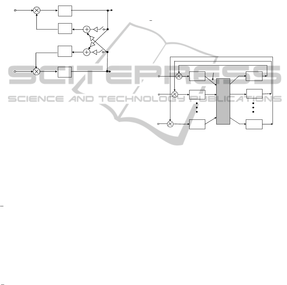
structure as shown in Fig. 3.
k
2
k
1
w
1
 w
1
w
0
w
0
LPF
G
1
V.C.O.
1
e
1
(t )
v
1
(t)
s
1
(t)
y
1
(t)
LPF
G
2
V.C.O .
2
e
2
(t)
v
2
(t)
s
2
(t)
y
2
(t)
s
i
(t) = A
Ci
sin(
i
t + Ψ
si
),
v
i
(t) = A
Vi
cos(
i
t + Ψ
i
); i = 1, 2.
Figure 3: The oscillating (PLL) neuron model.
It is easy to see that the model in Fig. 3. (PLL
model) consists of two antisymmetrically coupled
sinusoidal phase oscillators. The input signals s
i
(t),
i =1, 2 are sinusoidal carriers.
Thus:
s
i
(t) = A
Ci
sin(
i
t + Ψ
si
),
(23)
v
i
(t) = A
Vi
cos(
i
t + Ψ
i
); i = 1, 2.
(24)
Assuming ideal transmittances of loop filters, i.e.,
G
1
= G
2
≡ 1, the mean phase equation (Adler
equation) of this model is as follows (keys k
1
, k
2
open):
s1 1 s1 1
11V1m2 C2 V2
1V2m1C1V1
s2 2 s2 2 2
ΨΨ sin(ΨΨ) Δω
0wkkAA
d
2π
wk k A A 0
ΨΨ sin(ΨΨ) Δω
dt


  


  



  

(25)
where: Δω
i
- frequency deviations of the input s
i
(t)
signal
k
Vi
, k
mi
– sensitivity of VCO and phase-
detector, respectively
The similarity between Eq. (25) and the Kuramoto
model is worth noting. Closing k
1
, k
2
- keys in the
model from Fig. 3. one obtains an elementary PLL
orthogonal filter described by:
s1 1 s1 1
10 V1 m1 C1 V1 1 V1 m2 C2 V2
1 V2 m1 C1 V1 0 V2 m2 C2 V2
s2 2 s2 2 2
ΨΨ sin(ΨΨ)
Δω
-w k k A A w k k A A
d
2π
wk k A A -w k k A A
ΨΨ sin(ΨΨ) Δω
dt


  


  




  

(25)
where it is assumed that the connection matrix has a
form:
W
c
=W – w
0
1 (27)
with
W
2
= -1, W
T
= W
-1
= -W (28)
and w
0
> 0 (W –skew-symmetric, orthogonal)
Let us note that PLL implementation of the
elementary orthogonal filter from Fig.3. can be
easily scaled up to n-dimensional space. Such a
generalization is shown in Fig.4. (Citko and Sienko,
2008).
The Adler equation of this model is given by:
s1 1 s1 1
0v1m1 C1 v1 1v1m2 C2 v2 k-1v1mk Ck vk
s2 2 1 v2 m1 C1 v1 s2 2
2k-1 vk m1 C1 v1 0 vk mk C k vk
sk k sk
ΨΨ sin(ΨΨ)
wk k A A wk k A A w k k A A
ΨΨ wk k A A sin(ΨΨ)
d
2π
dt
wkkAA wkkAA
ΨΨ sin(Ψ
 
 




 








 





 

1
2
kk
Δω
Δω
ΔωΨ )











(29)
where : s
i
(t) = A
Ci
sin(
i
t + Ψ
si
)
v
i
(t) = A
Vi
cos(
i
t + Ψ
i
)
Δω
i
– frequency deviation
VCO
2
y
1
(t)
y
n
(t)
y
2
(t)
H
1
(s) VCO
1
H
2
(s)
H
n
(s) VCO
n
Connection
ma tr ix o f
PLL loops
s
1
(t)
s
n
(t)
s
2
(t)
input
output
Figure 4: A PLL model of the n-dim neural network.
Equation (29) can be rewritten as:

z = W
c
sin z + Δω
(30)
where: z = [z
1
, … , z
n
]
T
= [Ψ
s1
–Ψ
1
, … ,Ψ
sn
– Ψ
n
]
T
W
c
– matrix of connections.
It is worth noting that:
1. The hold range of a PLL network is
determined by the stable equilibrium of
Eq.(30). It means that, for a given Δω, one
can find loop gains (k
v
k
m
A
c
A
v
) such that
the PLL network attains synchronization in
the point: │sin z
i
│< 1, i = 1, … , n.
2. Under synchronization, the steady-state
output of the PLL network is given by:
y = sin z = W
c
-1
(– Δω). (31)
Taking the connection matrix W
c
as the
weight matrix in the orthogonal filter, the
output y gives the Haar spectrum of the
input vector. Moreover, the PLL network
from Fig. 4. can be treated as a n-
dimensional FM signal demodulator.
OscillatoryModelofNeuromorphicProcessorsbyEmbeddingOrthogonalFilters
331

3. The PLL network from Fig. 4. can be seen
as a model of the neural network with
dynamical connections. The weight of
connections can be changed by the
parameter k
v
(i.e. sensitivity of VCO).
4 OSCILLATORY MODEL OF
NEUROMOPHIC PROCESSORS
BY EMBEDDING
ORTHOGONAL FILTERS
By embedding the HNN-based orthogonal filters
into the net of PLL, one obtains a novel model of the
neuromorphic processor. Such a model is presented
in Fig. 5., where the structure from Fig.4. was
accordingly utilized.
y
1
y
2n
y
2
VCO
1
VCO
2
VCO
2n
Orthogonal filter with
weight matrix
-W+w
0
1
s
1
(t)
s
\2n
(t)
s
2
(t)
input
output
Figure 5: The oscillatory model of the neural network as
the embedded system.
It is worth noting that this model consists of the
network of "synaptic connections" hidden in the
structure of the orthogonal filter (Eq.4). Hence, it
could be a justification to name this structure as
neuromorphic. Moreover, the dynamic of the model
from Fig. 5 is given by Adler equations (29) and it
can be seen as a basic bulinding block to create the
oscillatory nets. The key contribution of this paper
can be formulated by the following statement: by the
chain connection of an even number of blocks from
Fig. 5. one obtains a ring structure performing
functions of self-sustaining memory with parallel
analysis of the input information by embedded
orthogonal filters.
A number of simulations were performed by
using Matlab-Simulink macro-models of phase
locked-loops. This analysis showed that oscillatory
memory proposed above exactly performed
algebraic functions of embedded orthogonal filters.
1
out
1
VCO
1
VCO
2n
Orthognal
filter 1
s
1
(t)
s
2n
(t)
1
2
2
out
2
VCO
1
VCO
2n
Orthognal
filter 2
Switch: 1 - input information
2 - memory
Figure 6: The self-sustaining memory ring with two
embedded orthogonal filters.
5 CONCLUSIONS
The main goal of this paper was to prove the
following statements:
An AI compatible processor should be
formulated in the form of a top-down structure via
the following hierarchy: the Hamiltonian neural
network (composed of lossless neurons) – the
octonionic module (a basic building block).
Furthermore, it has been confirmed that by using the
octonionic module based structures, one obtains
regularized and stable networks for learning. Thus,
typical for AI tasks, such as realization of classifiers,
pattern recognizers and memories, could be
physically implemented for any number N=2
k
(dimension of input vectors). It is clear that the
octonionic module cannot be ideally realized as an
orthogonal filter (decoherence-like phenomena).
Hence, the problem under consideration now is as
follows: how exactly an octonionic module be
realized by using cheap VLSI technology to
preserve the main properties -orthogonality, power
efficiency and scaleability. The possibility to
directly transform the integrator structure in to the
phase-locked loop (PLL)-based oscillatory structure
is noteworthy. It is clear, however, that oscillatory
neural network from Fig. 5. does not mimic the
biological spiking tissue. Nevertheless, we claim
that orthogonal filters-based data processing can be
considered as inspired by biological solutions.
REFERENCES
Citko, W., Sienko, W. (2008) Models of Oscillatory Nonlinear
Mappings
, Conference Proceeding of the First
International Workshop on Nonlinear Dynamics and
Synchronization (INDS08), July 18-19, pp. 170-176,
Klagenfurt, Austria.
Hoppenstead F. C., Izhikevich E. M. (1997)
Weakly
Connected Neural Network
, Springer, New York.
NCTA2014-InternationalConferenceonNeuralComputationTheoryandApplications
332

Hoppenstead F. C., Izhikevich E. M. (2000) Pattern
Recognition Via Synchronization in Phase-Locked
Loop Neural Networks, IEEE Transactions on Neural
Networks
, vol. 11, No.2.
Izhikevich, E. M. (1999)
Weakly connected quasiperiodic
oscillators, FM interactions, and multiplexing in the
brain, SIAM Journal on Applied Mathematics 59, pp.
2193-2223.
Izhikevich, E. M. (2006)
Dynamical Systems in
Neuroscience: The Geometry of Excitability and
Bursting, Cambridge, MA: The MIT Press.
Mcdonnell, M. D. et al. (2014)
Engineering Intelligent
Electronic Systems Based on Computational
Neuroscience
, Proceedings of IEEE, Vol. 102, No. 5,
p. 646.
Sienko, W. (1999)
Quantum Aspect of Passive Neural
Networks
, Proc. of Third International Conference on
Computing Anticipatory Systems, Liege, Belgium,
Sym. 2, p.18.
Sienko, W., Citko, W. (2009) Hamiltonian Neural
Networks Based Networks for Learning, In Mellouk,
A. and Chebira, A. (Eds.),
Machine Learning, ISBN
978-953-7619-56-1, J, pp. 75-92, Publisher: I-Tech,
Vienna, Austria.
Strogatz, S. H. (2000)
From Kuramoto to Crawford
exploring the onset of synchronization in populations
of coupled oscillators, Physica D 143: p. 1-20.
OscillatoryModelofNeuromorphicProcessorsbyEmbeddingOrthogonalFilters
333