Chirp Analyzer for Estimating Non-stationary Auditory Signals

Y. García-Puente

, P. Prado-Gutiérrez

1,2

and E. Martínez-Montes

Centro de Neurociencias de Cuba, La Habana, Cuba

Centro Interdisciplinario de Neurociencia de Valparaíso, Valparaíso, Chile

1 INTRODUCTION

The development of clinical tools for objectively

measuring the auditory temporal processing is

important for the early diagnosis of speech

pathologies related to hearing impairments. In this

regards, the use of mathematical models and signal

processing techniques is essential to characterize the

electrophysiological responses to speech-related

auditory stimuli. In this work, we present a Chirp

Analyzer (CA), as a new tool for the reliable

estimation of non-stationary auditory electro-

physiological responses. We study its properties and

potential applicability by comparing the estimated

responses with those obtained by standard time-

frequency methodologies, such as Short Time

Fourier Transform and Morlet Wavelet Transform.

2 METHODS

The Envelope Following Response (EFR) is an

auditory evoked potential elicited by acoustic stimuli

consisting in a carrier tone whose amplitude is

modulated by a chirp, i.e. a sinusoidal function with

a continuous sweep of amplitude modulation

frequencies. The physiological properties of the

auditory system suggest that the EFR strongly

depend on the modulation signal (chirp). Therefore,

the instantaneous estimated amplitude can be

considered a measure of the hearing ability to

response to each instantaneous modulation

frequency (IMF). (Purcell et al., 2004; Prado-

Gutierrez et al., 2012).

2.1 Simulated and Real Data

The simulated data consisted of a chirp with IMF

linearly varying from 20 to 120 Hz in each half as a

reference signal, multiplied by a simulated EFR

which imposes instantaneous amplitudes (envelope).

Here we simulated the EFR with different shapes

and delay (time difference between stimulus onset

and the electrophysiological response), adding in all

cases noise with signal-to-noise ratio SNR=2.

As real data, we used electrophysiological

recordings of adult rats, obtained in response to

amplitude-modulated carrier tones of 4 kHz. Stimuli

were delivered at 50 and 70 dB SPL. Chirp was

characterized by a linear sweep of IMF from 90 to

200 Hz in each half (15.36 s) of the stimulus.

Estimated EFRs were compared with the classical

EFR obtained with the Fourier Analyzer (FAM)

implemented in the MASTER system (Prado-

Gutierrez et al., 2012).

2.2 Short Time Fourier Transform

With the STFT, the non-stationary signal to be

analysed is divided into segments that can be

considered stationary. This uses a window function

gt,τ with fixed temporal width, which implies that

the temporal and spectral resolutions are the same in

the whole time-frequency plane. The STFT is

obtained as the Fourier transform of the product of

this window and the signal xt.

STFT



τ,



 xtgt,τe



(1)

In this work, we use the Goertzel algorithm to

estimate the STFT (discrete version) at

predetermined frequencies, using a Hamming

window (Boashash, 2003). With this method, the

EFR is obtained as the absolute value of the complex

coefficients in the time and frequency corresponding

to the stimulus’ IMF.

2.3 Morlet Wavelet Transform

The continuous wavelet transform (CWT) is defined

by:

CWT



τ,



xtW

,tτdt

(2)

Where, in our case, the function Wf,t is the

Morlet "mother wavelet":

W

,tσ



√

π

 

⁄















(3)

García-Puente Y., Prado-Gutiérrez P. and Martínez-Montes E..

Chirp Analyzer for Estimating Non-stationary Auditory Signals.

 2014 SCITEPRESS (Science and Technology Publications, Lda.)

where the temporal support σ



is inversely

proportional to the spectral support σ



(Boashash,

2003). The magnitude zf/σ



is kept constant.

Therefore, the spectral resolution is lower and the

temporal resolution is higher for increasing values of

IMF. This property makes CWT more attractive than

STFT for analyzing transient high-frequency

phenomena. The EFR is then extracted as the

absolute values of the wavelet complex coefficients

in times and frequencies corresponding to IMFs.

2.4 Chirp Analyzer

Instead of using a Fourier Basis, the chirp analyzer

(CA) proposed here consists in correlating the signal

xt with a non-stationary reference function φt

that represents the theoretical response:





xtgt,τφtdt

(4)

This procedure is carried out in overlapping

rectangular windows gt,τ, for achieving a higher

temporal precision with the same spectral resolution.

As this is done directly in the time domain, this

method is faster than the other methods that need to

estimate coefficients for all frequencies in each time

point. However, this also makes this method

sensitive to the phase difference between the signal

and the reference function, since correlation

vanishes when the signals are in counterphase. The

estimated EFR is extracted from values of CA in the

time points corresponding to each IMF.

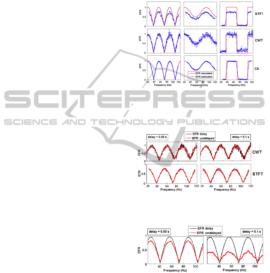
3 RESULTS

Figure 1 shows the response estimated by the three

methods (blue lines) for the simulated signals (red

lines) with different shapes, varying smoothness and

modulation depth. In all cases, the signals were

simulated with a peak signal-to-noise ratio SNR = 2

(noise variance is the half of signal´s maximum).

The first shape (left column) corresponds to a

sinusoidal squared response, with 100% modulation

depth; the second (central column) is a sinusoid with

50% modulation depth and the third (right column)

is a rectangular pulse with 100% modulation depth.

In real conditions, the auditory system responds

with a particular time delay with respect to the

stimulus onset, known as the latency of the response.

Moreover, the electronic equipment used for

recording the signals can introduce delays of up to

100 ms in some cases. Given that the methods

estimate the amplitude of the response at a particular

time, it is important to study how this delay affects

the estimated EFR with respect to the one obtained

using the exact latency of the response (hereinafter

called non-delayed response).

Figure 1: EFR estimation (blue line + dots) from simulated

signals with different shapes (red lines).

Figures 2 and 3 show the EFR estimated by the

three methods from data simulated with different

values of the response´s delay.

Figure 2: EFR estimated (red lines) with the CWT and

STFT from simulated signals with different values of the

auditory response´s delay, in comparison with the EFR

estimated for the non-delayed response (black lines).

Figure 3: EFR estimated (red lines) with the CA from

simulated signals with different values of the auditory

response´s delay, in comparison with the EFR estimated

for the non-delayed response (black lines).

In the analysis of electrophysiological recordings

in adult rats, the EFRs were obtained with the three

methods, as shown in Figure 4. For comparison

purposes, we plotted them normalized, together with

the EFR estimated with the Fourier Analyzer (FA)

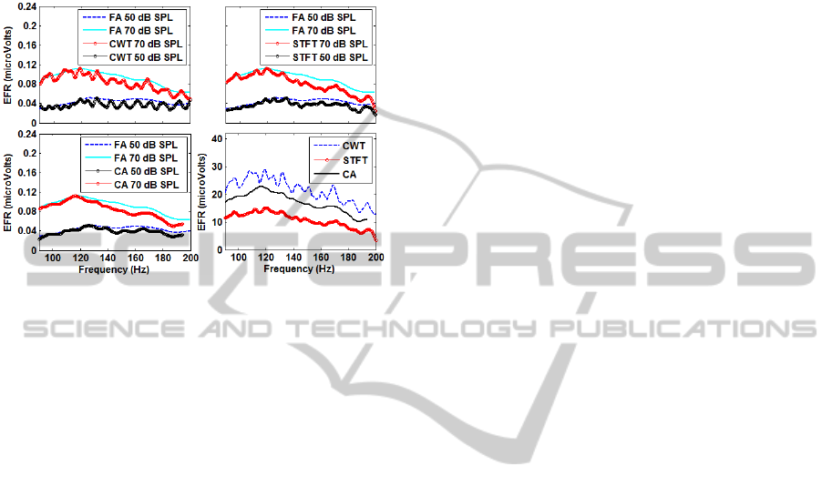
implemented in the stimulation and recording

system described in (Purcell et al., 2004; Prado-

Gutierrez et al., 2012). The bottom right panel of

figure 4 shows the estimated EFR without

normalization, which allows comparing the

responses’ amplitude obtained with each method.

Figure 4: EFR estimated from the real electrophysiological

recordings in adult rats. Top row and bottom left:

responses were normalized such that all maxima coincide

with that of the classical Fourier Analyzer (FA). Bottom

right: non-normalized responses estimated with the three

methods.

4 DISCUSSION

Although the three methods were able to recover the

shape of the simulated responses, some interesting

differences were evident (Figure 1). CWT and CA

estimated the amplitude with higher accuracy, but

the former is more sensitive to noise and therefore,

overestimates the amplitude of small or null

responses. This is explained by the higher temporal

(and lower spectral) resolution of the CWT in the

frequency band studied. The STFT did not estimate

the amplitude correctly (underestimating it), due to

the violation of the main assumption of this method,

i.e. the stationarity of the signal (Boashash, 2003).

Also, the rectangular pulse showed that the CA

reflected the abrupt changes in the response with

slightly lower temporal resolution than the CWT.

Figures 2 and 3 showed that the EFR estimated

with the CWT was the less affected by changes in

the response´s delay. Again, this is explained by its

lower spectral resolution for high frequencies, which

leads to similar amplitudes of the response in a wide

time-frequency range. Contrarily, the higher spectral

resolution of the STFT led to great changes in the

amplitude estimated in nearby time-frequency

points. The CA is the most affected when the

response is estimated by selecting the wrong time-

frequency points, since this method rely in

correlating the signal with a reference function. The

delay corresponds to a phase difference between

both signals, which makes the correlation to drop

drastically (Figure 3).

Results of the analysis of real data showed that

the three methods may be considered as useful tools

for the estimation of non-stationary auditory evoked

responses. The EFR estimated showed similar

shapes than the one obtained with the FA, which is

one of the most popular methods to study this type

of auditory responses (Purcell et al., 2004; Prado-

Gutierrez et al., 2012). The CWT presented higher

variability and more local extremes, due to its

sensitivity to noise. However, this effect can be

ameliorated by smoothing the response in a post-

processing (e.g. we used a 7-point sliding window

smoother). Regarding the non-normalized responses,

the STFT showed the smallest amplitudes. Also,

amplitude of the EFR estimated with the CWT was

higher than those of the CA for all frequencies,

which suggests the existence of a response delay.

In summary, among the three methods studied

here, the CA is the fastest (around 3s against more

than 30s each of the other two approaches) and most

reliable method to estimate the amplitude of the

EFR. However, this method is strongly affected

when the latency of the response (together with

electronic delays) is high. As this value is usually

unknown, this method should be used carefully and

new ways of estimating the response’s delay have to

be the goal of future developments. All these results

suggest that the CA is a promising tool to estimate

the EFR, although optimal estimation could be

achieved with a methodology that combines the

good properties of the three techniques.

REFERENCES

Prado-Gutierrez P, Mijares E, et al. (2012) Maturational

time course of the Envelope Following Response to

amplitude-modulated acoustic signals in rats.

International Journal of Audiology 51(4): 309-316.

Purcell DW, John MS, et al. (2004) Human temporal

auditory acuity as assessed by envelope following

responses. J AcoustSoc Am 116(6): 3581–3593.

Boashash, B (2003) Time frequency signal analysis and

processing. Elsevier, London.