
Sentiment Polarity Extension for
Context-Sensitive Recommender Systems
Octavian Lucian Hasna, Florin Cristian Macicasan, Mihaela Dinsoreanu and Rodica Potolea
Computer Science Department, Technical University of Cluj-Napoca, Gh. Baritiu st. 26-28, Cluj-Napoca, Romania
Keywords: Sentiment Detection, Meta-Features, Classification, Text Mining, Design and Implementation, Evaluation.
Abstract: Opinion mining has become an important field of text mining. The limitations in case of supervised learning
refer to domain dependence: a solution is highly dependent (if not specifically designed or at least
specifically tuned) on a given data set (or at least specific domain). Our method is an attempt to overcome
such limitations by considering the generic characteristics hidden in textual information. We aim to identify
the sentiment polarity of documents that are part of different domains with the help of a uniform, cross-
domain representation. It relies on three classes of original meta-features that can be used to characterize
datasets belonging to various domains. We evaluate our approach using three datasets extensively used in
the literature. The results for in-domain and cross-domain verification show that the proposed approach
handles novel domains increasingly better as its training corpus grows, thus inducing domain-independence.
1 PROBLEM STATEMENT
In the past years, the popularity of online reviews as
a decision support system grew. We start to base our
daily decisions on the information they reflect.
Whether it’s a new laptop, the destination of a
vacation or where to apply for a master’s program,
our information needs are driven by the experiences
of others before us. Furthermore, online reviews are
a source of insight for companies that look for early
customer feedback (The Economist, 2009). In this
context, an automated solution for tagging reviews
with their sentiment orientation is beneficial.
We propose an approach to document-level
sentiment polarity identification that leverages a
combination of three meta-feature classes. The
novelty of the approach relies on the feature-vector
characteristics: as the classification instances are
characterised via meta-features, the model gains in
generality being domain quasi-independent.
We utilise the following three classes of meta-
features:
Part-of-speech patterns represent syntactic
constructs with increased sentiment promise;
Polarity histograms group the words of a
document in buckets based on their sentiment
polarity;
Sentiment lexicons represent a proven
collection of words annotated with polarity
information.
We incorporate the sentiment polarity identifier
in a context-sensitive recommendation workflow.
The aim of this use-case is to associate to an input
collection of unstructured documents (context) the
most appropriate content. We define the content as a
document already structured and tagged. Documents
are tagged with their sentiment polarity as a result of
the classification based on meta-features.
Furthermore, a thematic reference system brings
structure to the context. Both of these aspects are
combined to generate a recommendation.
2 RELATED WORK
In (Liu, 2012) three dimensions of sentiment
analysis are underlined: document, sentence and
aspect. A document-level analysis is interested in the
whole expressed opinion. The implicit assumption is
that the entire document expresses an opinion on a
single entity. Sentence-level analysis is closely
related to subjectivity classification. It requires the
identification of subjective views and opinions. At
aspect-level, sentiment is expressed with respect to
various components of an entity. Entity features are
selected from frequent nouns or noun phrases and
126
Hasna O., Macicasan F., Dinsoreanu M. and Potolea R..
Sentiment Polarity Extension for Context-Sensitive Recommender Systems .
DOI: 10.5220/0005141101260137
In Proceedings of the International Conference on Knowledge Discovery and Information Retrieval (KDIR-2014), pages 126-137
ISBN: 978-989-758-048-2
Copyright
c
2014 SCITEPRESS (Science and Technology Publications, Lda.)

their sentiment orientation is measured using
lexicon-based approaches. The same conceptual
feature can be represented with different textual
representations. This is why synonyms become an
important tool for aspect-based sentiment analysis.
At the core of each approach is identifying the
sentiment orientation of individual words.
In (Socher, et al., 2013), they are interested in
analysing the sentiment orientation of short phrases,
like Twitter comments. The goal is to analyse the
compositional effect of sentiment in a given short
phrase. To this purpose they propose the Sentiment
Treebank, a corpus of labelled parse trees. It
leverages the Recursive Neural Tensor Network
model that represents a phrase through a word vector
and a parse tree. A tensor-based compositional
function is used to associate sentiment polarity to
individual tree nodes. The consolidated polarity of
the root gives the orientation of the phrase. They
leverage seven sentiment orientations (three degrees
of negative, neutral and three degrees for positive).
In (Liu, et al., 2012), they propose a set of
heuristics for extracting expressions with increased
sentiment affinity based on dependency relations.
They focus on range, trend and negation indicators.
The range indicators are viewed as the members of
the WordNet synset of “above” while trend
indicators are modelled around “increase”.
Furthermore, they detect negation and cluster part-
of-speech and grammatical relations to increase
generality.
In (Lin, et al., 2012) they propose a probabilistic
modelling approach to sentiment detection. Their
Joint Sentiment-Topic Model (JST) is based on latent
Dirichlet allocation (LDA) (Blei, et al., 2003). Apart
from the thematic representation, documents in JST
get also a sentiment label.
Ensemble techniques for sentiment classification
are explored in (Xia, et al., 2011). Feature sets and
classification algorithms are integrated with the aim
of improving accuracy. They define three POS-
based feature classes: adjectives (JJx), nouns (NNx)
and verbs (VBx). Furthermore, they utilize word
dependency parsing together with unigrams and
bigrams as WR-based feature sets.
Domain independent sentiment lexicons are used
in the work of (Ohana, et al., 2011) in order to tune a
classifier on different domains. They propose both
fix scoring schemas and sum-based predictors that
boost results on the analysed domains. Class-
imbalanced recall is viewed as an issue for scenarios
when misclassification costs vary with class. They
propose a term frequency-based score adjustment
metric as a possible solution.
The problem of domain adaptation is investigated in
(Blitzer, et al., 2007). They propose a
correspondence technique for learning structural
similarities between lexicons specific to different
domains. In (Raaijmakers & Kraaij, 2010) the
problem of domain adaptation is approached by
using an annotated subset of the target domain to
tune a single-domain classifiers.
3 TERMINOLOGY
In the following we formally define the basic
notions used throughout the article.
The sentiment polarity of an entity
describes an ordered distribution over
orientations: Positive, Negative,
Objective such that
〈
,,
〉
where 1;
The sentiment orientation of an entity
(
∈
0,,
) is described as
argmax
∈
x
A word w is the basic unit of discrete data
(Blei, et al., 2003), defined to be an element
of a vocabulary V. A word can have a
sentiment polarity
;
A document
,
,…,
is a
sequence of words in any language;
A keyword is a word of a document
having high descriptive value. Let
represent all the keywords of document d;
A context is defined by a collection of
weighted documents of arbitrary structure;
〈
,
〉|
∈
, where
∑
∈
1;
The content is defined by a collection of
labelled documents which have a well-
defined structure. Each document has a
sentiment polarity
and a distribution
over topics (Dinsoreanu, et al., 2012);
〈
,
,
〉|
∈
4 SYSTEM ARCHITECTURE
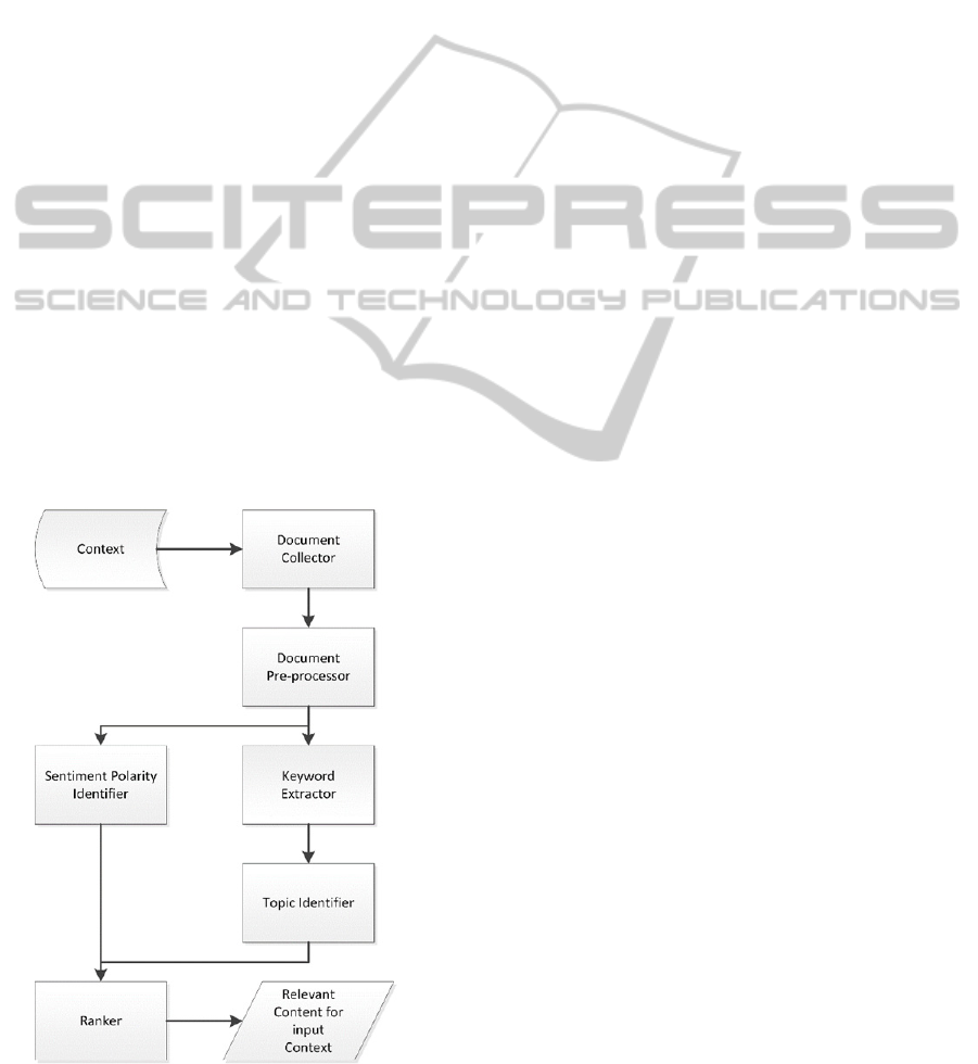
Functional Description of the Modules: Our
architecture (Figure 1) consists of six main modules
that interact to generate sentiment-aware
recommendations.
The first module, Document Collector (DC)
acquires documents describing the context and
extracts their textual information. The documents
lack structure and can contain text in any language.
SentimentPolarityExtensionforContext-SensitiveRecommenderSystems
127
This is why we first identify the language. If the
detected language cannot be machine-translated into
English then the document is rejected.
(1)
The second module, Document Pre-Processor
(DP) performs an initial syntactic analysis on a
single document from the context collected by DC.
It tokenizes collected documents into sentences and
words. Furthermore, it annotates each such word
with their corresponding part-of-speech. Finally, it
filters out tokenization by-products like raw
numbers or punctuation that served their purpose
once the part-of-speech tags are in place. Let d be a
document from
.
(2)
The Sentiment Polarity Identifier (SPI) detects
the sentiment polarity for the given document () by
analysing its associated collection of words (
).
This analysis extracts domain-independent meta-
features that are further used to decide the proper
orientation.
(3)
The Keyword Extractor (KE) and Topic Identifier
(TI) are functionally equivalent with the modules we
leveraged in our previous work (Dinsoreanu, et al.,
2012). KE reduces
to a set of elements with
increased descriptive value.
Figure 1: Conceptual Architecture.
TI leverages its underlying topic model in order to
associate to each
a distribution over topics
via
topic-level unification. The two modules are
formally described as follows:
(4)
(3)
The Ranker (R) filters documents from
with respect to performance criteria (Γ). We aim for
recommendations that match the sentiment polarity
and are thematically close to the documents
from
.
argmax
∈
Γ
(6)
5 META-FEATURES FOR
SENTIMENT CLASSIFICATION
Our approach aims to achieve domain-independence
by inferring sentiment polarity using meta-features.
The goal is to generalize the members of the feature
vector so as not to bind them to the characteristics of
a specific domain. We employ three main classes of
features: sentiment lexicons, part-of-speech patterns
and polarity histograms.
5.1 Sentiment Lexicons
A sentiment lexicon (SL) is represented by a
collection of words annotated with their sentiment
polarity. Formally it can be described as follows:
〈
,
〉|
∈
(7)
We also define the basic operations (union,
intersection and difference) on sentiment lexicons.
An operation applied on a SL is equivalent with
applying that operation on their associated
vocabulary. In case of vocabulary overlaps,
collisions are resolved by selecting the sentiment
polarity of the SL with the highest priority (an
input). Thus, we define the following:
∪
〈
,
,
〉
∈
∧
,
(8)
∩
〈
,
,
〉
∈
∧
,
(9)
∖
〈
,
,
〉
∈
∖
(10)
Our approach uses as lexicon a combination
between two collections commonly used in
literature. The first lexicon is proposed in (Hu &
KDIR2014-InternationalConferenceonKnowledgeDiscoveryandInformationRetrieval
128

Liu, 2004) and represents a list of positive and
negative sentiment words for English. Depending on
orientation, we associated to each word in this
lexicon one of the following polarities:
〈
0.9,0.05,0.05
〉
or
〈
0.05,0.9,0.05
〉
. We
denote this sentiment lexicon as
.
The second resource we leverage is
SentiWordNet (SWN) (Baccianella, et al., 2010).
SWN is the result of an automatic annotation of all
WordNet synsets (ss). As a result, each synset
receives a positive and a negative polarity. SWN
uses the WordNet structure which groups similar
meanings of different words in a synset. A word can
be part of multiple synsets by exhibiting a different
sense. So a word can have different sentiment
polarities based on the sense it plays in the analysed
document. Let
be the set of synsets
associated to a word in SWN.
In order to build a sentiment lexicon associated
to SWN (
) we need to associate a single
polarity to each word. Words might be associated
with multiple synsets (
|
|
1). This is why
we define the multi-synset fall-back schema (MSFB)
which associates to each word a polarity. Either their
synset’s if the word is part of a single synset or the
polarity of the synset that maximizes the absolute
difference between their positive () and negative
() polarity. This relation is defined as follows:
〈
,
〉|
∈
(4)
MSFB
∈
(5)
Since many of the synsets are objective we
choose to define dSWN as the subset of SWN with
synsets that have a distinguishable positive or
negative polarity. Thus, we define
∈
〈
,,
〉
∧
∧
∨
(6)
This reduces the number of synsets and helps us
underline the sentiment baring words. A sentiment
lexicon
is strongly distinguishable if, for any
∈ the condition (6) stands (
is also
strongly distinguishable).
Applying MSFB, we build
as the
sentiment lexicon associated to dSWN. An
interesting consequence is that the percentage of
words with a single synset grows. Furthermore, we
are interested in analysing the vocabulary overlap
between
and
. With the help of
relations (8), (9) and (10) we can further refine
lexicon combinations.
We leverage sentiment lexicons as domain-
independent meta-features. They represent a fixed
set of words that are to be searched in document
instances. We measure a Boolean meta-feature (i.e.
whether or not an element of the lexicon appears in
the document instance). The feature vector
associated to a
is described as follows:
d
1,∈
0,∉
∈
(7)
Another interesting aspect of sentiment lexicons
is negation. Any word might appear in a negated
context which inverses its sentiment polarity:
〈
,
,
〉|
∧
∧
(8)
In the rest of the article, we will refer to
combinations between sentiment lexicons based on
the applied set of operations (e.g. the union between
and
becomes
_∪_
).
5.2 Part-of-Speech Patterns
Part-of-speech patterns (
,
) repre-
sent a specialized combination of words tagged with
POS information. In (Turney, 2002) five such
patterns are used to extract bigrams with increased
sentimental promise. He analyses trigrams that
respect the part-of-speech patterns represented in
Table 1 and selects bigrams based on the priority
induced by the third word (the first POS pattern has
a higher priority than the next three.
Table 1: POS patterns proposed by Turney.
i
First Word
POS (
)
Second Word
POS (
)
Third Word
(not extracted)
1 Adjective Noun Anything
2 Adverb Adjective Not Noun
3 Adjective Adjective Not Noun
4 Noun Adjective Not Noun
5 Adverb Verb Anything
A bigram (
〈
,
〉
) will match the i
th
part-of-
speech pattern (
) if the following relation
stands:
,
〈
〉
≡
(9)
We propose the usage of these patterns as meta-
features in two instantiations. One for the positive
orientation (
) and one for the negative
(
) thus generating 10 meta-features.
The polarity of a POS pattern is computed based
on a linear combination between the sentiment
polarities of the two words that are part of the
SentimentPolarityExtensionforContext-SensitiveRecommenderSystems
129
pattern. Instances with a distinguished positive
polarity count for
. If the negative polarity is
distinguished it will count for
. We describe
the relation as follows:
,
∗
1
∗
(10)
where is an experimentally computed coefficient
and
and
are retrieved from a sentiment
lexicon. We’ve determined that a good would be
0.5 for
and
. For the other three, we
associate 0.8 for the adjective or adverb. We treat
negation for by considering
,
as the pattern’s polarity.
The count of an individual instance in a
document is described as follows:
,,
∈
,
,
(11)
where
is a word from where the i
th
pattern is
instantiated with the proper sentiment orientation.
For each document, we compute the part-of-
speech patterns feature vector as a 10-tuple
described by the following relation:
,,
1,5
,∈
,
(12)
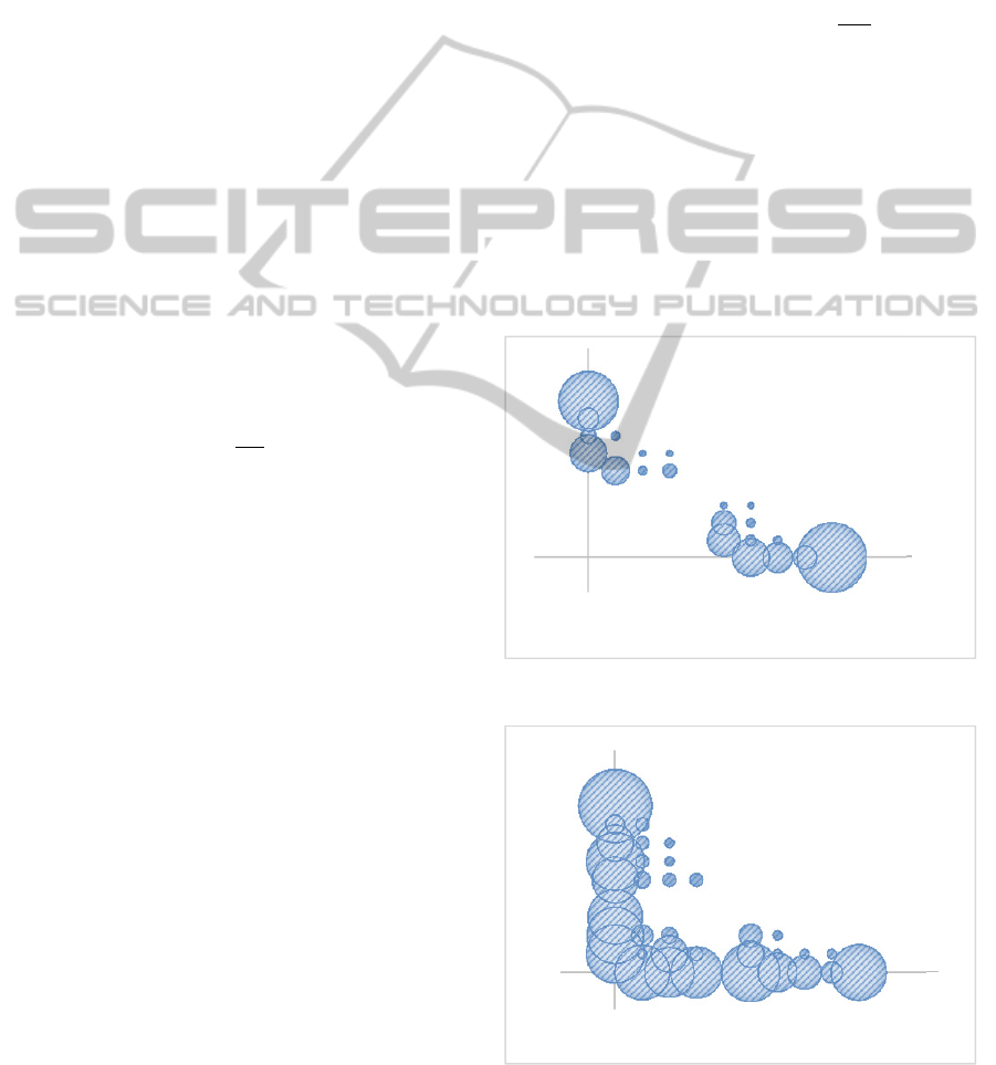
5.3 Polarity Histograms
Polarity Histograms are a measure of the degree to
which a document contains words of different
sentiment polarities. We analyse words from the
document that exhibit sentimental promise based on
the polarity lexicon. We group them in buckets of
size ∆ on a two-dimensional lattice. The actual
bucket size depends on the polarity values reported
by the sentiment lexicon.
The diameter of a disc in Figure 2 and Figure 3
represent the number of words that have a positive
sentiment polarity within ,∆
and a negative
polarity within,∆
.
Figure 2 depicts the polarity histogram of a
positive document. It uses
_∪_
as
sentiment lexicon. There are no words in buckets
bellow 0.5 because the lexicon is strongly
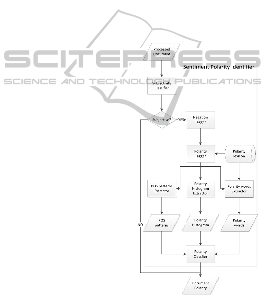
distinguishable. In Figure 3, we represent the
polarity histogram resulted from processing a
negative document using the
_∪_
lexicon.
The lexicon used for this document lacks the
distinguishability property.
We adopt polarity histograms as the third set of
meta-features as they capture the overall polarity
information of a document, normalized to a given
lexicon. In the polarity context, negations have the
same impact as for POS patterns. Thus, we inverse
the sentiment polarity for a word if it occurs negated
in the document. In our experiments, the total
number of buckets is 66 (as describe in relation
(13)).
66
〈
,0.1
,
,
0.1
〉
1
∗0.1
∗0.1
,0,10
(13)
The size of an individual bucket is measured as
follows:
,
∈
∧
∈
(14)
where
is a word from and its sentiment polarity
falls within the .
The polarity histogram feature vector that
corresponds to a document is described as follows:
,
|
∈
(15)
Figure 2: Polarity histogram for a document with positive
sentiment orientation using
_∪_
.
Figure 3: Polarity histogram for a document with negative
sentiment orientation using
_∪_
.
‐0,2
0
0,2
0,4
0,6
0,8
1
1,2
‐0,2 0 0,2 0,4 0,6 0,8 1 1,2
Negativepolarity
Positivepolarity
‐0,2
0
0,2
0,4
0,6
0,8
1
1,2
‐0,2 0 0,2 0,4 0,6 0,8 1 1,2
Negativepolarity
Positivepolarity
KDIR2014-InternationalConferenceonKnowledgeDiscoveryandInformationRetrieval
130
6 SENTIMENT-AWARE
RECOMMENDATIONS USE
CASE
We analyse the problem of associating a sentiment
orientation to a document in relation to a context-
aware recommendation system. Unstructured input
context is analysed and tagged with both a sentiment
polarity and a thematic distribution. These values are
combined in order to detect the most appropriate
structured content.
6.1 Pre-Processing
We split our pre-processing effort into two levels: a
corpus-level collector and a document-level pre-
processor.
We start with the Document Collector flow
which acquires a corpus (collection of documents)
describing the context. We reduce each document to
plain text. HTML documents are filtered for
removing tags. The inner plain text is extracted from
the cleaned document and annotated with source
tags. Language detection is applied on plain text. We
attempt to detect the language of the acquired corpus
using the Autonomy-IDOL API. In case of a
successfully language detection the machine
translation using the Google Translate API is
applied (in case the language is not English). Next,
the specialized pre-processing analysis is performed.
To properly extract the three types of meta-
features and to prepare the keyword candidates, a
document-level analysis within the Document Pre-
processor is performed. The documents are split
into sentences and sentences into words using a
tokenizer that mimics Penn Treebank 3 (Marcus, et
al., 1999) tokenization. Each token is annotated with
part-of-speech information using a log-linear tagger.
Both operations are incorporated into the Stanford
POS Tagger (Toutanova, et al., 2003). Then, we
remove noise by filtering out non-word entries.
6.2 The Sentiment Polarity Identifier
The Sentiment Polarity Identifier (SPI) in Figure 4
is responsible for associating a sentiment polarity
(
) to a document ().
The first step of the polarity identification
process is deciding whether or not the input
document is subjective. This helps us filter out
objective documents (their sentiment analysis is
outside the scope of this work). To this purpose, we
adapt the work of (Lin, et al., 2012) for the task of
subjectivity detection. They propose the Joint
Sentiment-Topic model (JST) as an extension to
LDA.
The generative process for JST follows three
stages. One samples a sentiment label from a per-
document sentiment distribution. Based on the
sampled sentiment label, one draws a topic from the
sentiment-associated topic distribution. Finally one
chooses a word from the per-corpus word
distribution conditioned on both the sampled topic
and sentiment label. In order to infer the latent
thematic structure, they use a collapsed Gibbs
sampling approximation technique. We built upon
their approach a binary classifier that is responsible
for analysing the distribution over sentiment labels
of an input document.
Figure 4: Sentiment Polarity Identifier.
SentimentPolarityExtensionforContext-SensitiveRecommenderSystems
131
Subjective documents are further analysed with
respect to the three classes of meta-features. To
better measure the sentiment orientation of a word,
we start with negation detection for which a naïve
approach is applied, that searches for words that are
part of a negation lexicon. So far only explicit
negations are considered (words negated by not,
don’t and similar). Each time such a word is
detected its determined word is marked as negated.
Next, the polarity tagging step attaches to each
processed word its associated sentiment polarity
using the configured sentiment lexicon. The polarity
of the document is aggregated from the document’s
words which belong to the lexicon as well. The
sentiment polarity of a word is inversed if it is
preceded by a negation. Polarity enriched words are
the input for all three meta-feature extractors.
At this point we start collecting instances of our
three meta-feature classes. The POS patterns
extractor collects instances of the 10 POS patterns.
Then we apply the polarity histogram extractor
which starts filling in the defined buckets based on
the individual polarity of words in the analysed
document. Finally, we apply the polarity words
extractor that selects the words that are part of the
sentiment lexicon. At this level, we treat negation by
doubling the size of the lexicon’s vocabulary (each
word gets negated).
The feature vector of a document (fvd) used by
the polarity classifier is formally described as
f
v
⋃
⋃
.
(16)
It contains the following meta-features:
10 meta-features whose values represent the
number of part-of-speech pattern instances
of each type found in the document;
For each polarity histogram bucket, the
number of words with
within that
bucket;
For each word in the polarity lexicon, a
Boolean marker describing its membership
in
.
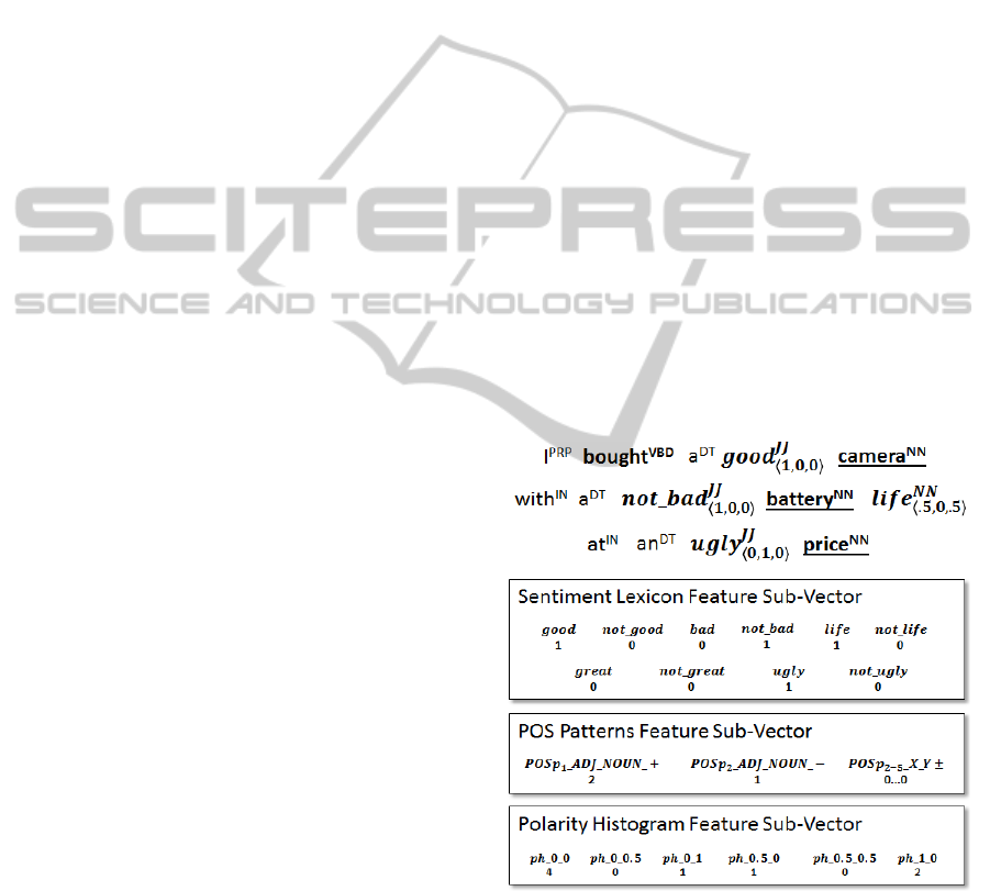
In Figure 5 we detail the three main components
of the feature vector generated by analysing a toy
sentence. In this toy example, the sentiment lexicon
contains 5 polarized words (good, bad, life, great
and ugly) together with their negation. The
associated sub-vector marks their presence in the toy
sentence. Furthermore, three
instances are
detected (the underlined noun together with the
adjective on the left). Two of the instances have a
positive orientation as opposed to “ugly price”
which is a negative instance. For the polarity
histogram, we chose ∆0.5 which generates 6
buckets. Four words are objective (“bought”,
“camera”, “battery” and “price”), one is strongly
negative (“ugly”), two are strongly positive
(“not_bad” and “good”) and one is partially positive
(“life”).
6.3 The Context-Sensitive
Recommender
The interaction between the Keyword Extractor
(KE) and the Topic Identifier (TI) generates
context-sensitivity.
The Keyword Extractor reduces the vocabulary
of a processed document to words with high
descriptive value. We build upon previous work
(Dinsoreanu, et al., 2012) by refining the keyword
model and features. This module performs another
processing step that prepares the candidates for
keyword status by annotating them with the features
used in the classification step. First, it removes the
stop-words and then transforms all the words to their
lemma using the WordNet lexicon. After that it
replaces all the synonyms with a “representative
synonym” using the same lexicon. Then it computes
the occurrence, frequency and tf-idf values for every
word. Furthermore, we now consider part-of-speech
information as a discriminative feature.
Figure 5: Instances of meta-features in a toy sentence.
Finally a candidate for a keyword has the
following features for a plain text document:
hasCapitalLetters which is true if the
candidate has at least one capital letter;
firstPosition which gives the first appearance
of the candidate in the text;
KDIR2014-InternationalConferenceonKnowledgeDiscoveryandInformationRetrieval
132

relativeFirstPosition which is computed as
the division between firstPosition and the
number of words in the document;
occurrence, frequency, tf-idf;
part-of-speech.
If the document is in HTML format then the
candidate has a couple more features: inPageUrl,
inTitle, inMetaDescription, inHeadings, inLink
Name, inImageAlt.
Finally all the meta-features are sent to the
Keyword Classifier and this sub component selects
the keywords.
The Topic Identifier builds its underlying
thematic model by associating to each document a
distribution over topics (
). We refer the reader to
(Dinsoreanu, et al., 2012) for a detailed description
of this module.
The Ranker selects the best document (
) as
the document with the maximum priority (
) in the
context. This can be expressed as:
argmax
∈
(17)
Then it applies SPI for determining sentiment
polarity (
) and TI for computing topic
distribution (
). Furthermore, it computes the
sentiment orientation (
). Finally, it searches for
documents in
which are similar with the
topic distribution (
) and have the same sentiment
orientation (
). In our previous work, we
determined that a good threshold () for the
similarity between
is 0.7.
∈
∧
,
∧
(18)
7 RESULTS AND EVALUATION
7.1 Sentiment Classifier
We are first interested in the effect of applying the
distinguishability property on
. We analyse
the dimensionality reduction induced by this
property with a focus on the proportion of words that
end up being associated with a single synset. In
Table 2: Comparison between SWN and dSWN we
show the number of synsets (#syn) and words (#w)
in both sentiment lexicons.
has 94.1% less
words and 95.1% less synsets then
.
Furthermore, we measure the distribution of words
(SynPerWord) that are associated to a single synset,
2 or 3 synsets or more. Table 2 shows that for 85.4%
of the words from
a unique sentiment
polarity can be associated from their corresponding
synset. This means that we rely on the multi-synset
fall-back schema (relation (5)) 4 times less than
for
.
Table 2: Comparison between SWN and dSWN.
#syn #w
SynPerWord
1 2or3 more
SWN 117659 147306 .401 .124 .475
dSWN 5736 8548 .854 .134 .012
The third aspect that we analyse is the best
configuration for the feature vector. Based on
preliminary results for initial evaluations on
different classifiers (NB, SVM and C4.5), we
restricted the evaluations to the Naïve Bayes
(implementation available in Weka) configured to
use a kernel separator (Witten, et al., 2011). While
evaluating the configuration of the classifier we use
the version 2.0 of the Movie Review Dataset (MR)
first introduced by (Pang & Lee, 2004). It consists of
1000 negative and 1000 positive movie reviews
crawled from the IMDB movie archive. The average
document length is 30 sentences.
For validation, we randomized the dataset, hid
10% for evaluation and split the remaining 90% into
10 folds. The classifier is trained 10 times on 9
different folds (81% of the corpus), tested on 1 fold
and evaluated against the hidden 10%. We repeat
this process with multiple random seeds.
The evaluations were performed on the data set
with different features combinations. The first set of
features is the elements of a sentiment lexicon. The
candidate lexicons are
,
and the
lexicons obtained by applying the basic set
operations on the two (denoted correspondingly in
Table 3 and Table 4). By structurally analysing the
lexicons, we measured the number of words (#w) in
each and the distribution of positive (#pw) and
negative (#nw) word sentiment polarities. In Table 3
we compare the lexicon candidates with respect to
their vocabulary size. It’s interesting to note for all
lexicons the distribution of negative words is greater
than the distribution of words with a positive
sentiment orientation.
Table 3: Sentiment lexicon operations comparison.
#w #pw #nw
6786 .295 .705
8548 .359 .641
_
∪
_
13080 .336 .664
_
⋂
_
2254 .302 .698
_
∖
_
4532 .291 .708
_
∖
_
6294 .380 .620
SentimentPolarityExtensionforContext-SensitiveRecommenderSystems
133

Using only such features while classifying instances
from MR we measured the average weighted
precision and recall for the positive and negative
classes together with their standard deviation. The
results in Table 4 suggest that the best sentiment
lexicon choice is the union between the two
lexicons. Furthermore, the vocabulary intersection
sub-set is more valuable than any of the sub-sets
specific to one of them.
Table 4: Lexicons evaluation.
awp
awr
.755 .026 .746 .026
.727 .016 .724 .016
_∪_
.767 .029 .758 .029
_⋂_
.711 .013 .708 .014
_∖_
.668 .025 .664 .026
_∖_
.629 .021 .627 .018
Next the evaluation is seeking for finding the
best feature set, using as candidates our three meta-
feature categories, part-of-speech patterns (POSP),
polarity histograms (PH) and the sentiment lexicon
(SL). Seven experiments were performed each
considering a different combination of the three
categories of feature vector candidates. For polarity
histograms we set the bucket sizes ∆
and ∆
to 0.1.
The results in Table 5 show that each of the three
meta-feature classes brings an incremental
improvement. The biggest impact is brought by the
sentiment lexicon. The best feature vector contains
the combination between part-of-speech patterns,
polarity histograms and the sentiment lexicon.
Table 5: Feature vector composition from meta-features.
Configuration awp
awr
POSP .642 .027 .637 .031
PH .640 .029 .624 .028
SL .767 .029 .758 .029
SL + POSP .816 .014 .814 .014
SL + PH .825 .016 .820 .016
PH + POSP .671 .027 .664 .033
SL + POSP + PH .841 .015 .829 .016
To asses domain independence we have tested
the feature vector configuration on other domains.
Proposed by (Blitzer, et al., 2007), the Multi-
Domain Sentiment (MDS) dataset is a collection of
Amazon reviews from multiple domains. It consists
of 26 domains with labelled positive and negative
reviews. We’ve considered in our experiment 14
domains that have more than 800 positive and 800
negative labelled reviews. In literature, the initial 4
domains are extensively used for evaluation. They
cover the Book (B), DVD (D), Kitchen (K) and
Electronics (E) and have 1000 positive and 1000
negative reviews. For this experiment we also
measure classification accuracy (acc) because this is
the metric used for comparison in other studies using
the MDS-4. Table 6 reports the results for 10
random seeds with two outliers excluded (min &
max awp) on both MR and the 15 domains of MDS.
The relative balance of the measured precision and
recall (0.8% difference) suggest that our approach
does not affect sensitivity and is able to consistently
identify polarity in different domains.
Table 6: In-domain verification using multiple domains.
Dataset awp
awr
acc
MR .841 .015 .829 .016 82.87
Book (b) .740 .025 .712 .029 71.89
DVD (d) .807 .023 .800 .026 80.03
Electro (e) .801 .025 .796 .024 79.59
Kitchen (k) .849 .019 .847 .018 84.69
Apparel (a) .853 .019 .851 .019 85.12
Baby (ba) .837 .022 .836 .021 83.62
Camera (c) .855 .022 .851 .023 85.13
Health (h) .810 .025 .808 .024 80.86
Magazine (m) .857 .018 .852 .019 85.26
Music (mu) .792 .023 .789 .024 78.99
Software (s) .825 .029 .818 .032 81.87
Sports (sp) .819 .026 .816 .027 81.67
Toys (t) .829 .021 .825 .023 82.57
Video (v) .762 .038 .741 .047 74.10
AVERAGE .818 .040 .811 .046 81.21
We compare our approach with other studies that
leveraged the same datasets for in-domain
classification (training and validation on the same
domain). In Table 7 we compare against the results
of in-domain testing of (Lin, et al., 2012),
(Raaijmakers & Kraaij, 2010) and (Blitzer, et al.,
2007) and against the results obtained with NB from
(Xia, et al., 2011).
Table 7: Accuracy comparison with literature.
MR B D E K
Lin2012 76.6 70.8 72.5 75 72.1
Xia2011P
oS
82.7 76.7 78.85 81.75 82.4
Xia2011
WR
85.80 81.2 81.7 84.15 87.5
RK2010 N/A 78.8 82.3 86.5 88.8
Bli2007 N/A 80.4 82.4 84.4 87.7
Proposed 82.87 71.18 80.03 79.59 84.69
We are further interested in experimenting with
cross-domain verification. We split all the domains
() into 10% for validation and 90% for training
using different random seeds. This will generate an
in-domain test (used as “golden standard”) and
KDIR2014-InternationalConferenceonKnowledgeDiscoveryandInformationRetrieval
134

1 cross-domain tests (test on other domains).
Table 8 covers our results. The datasets are
referred to by their initials from Table 6. We
measure the relative loss () in classification
accuracy due to cross-domain verification. Let
the accuracy of training on domain train and
testing on domain test. Thus the relative loss
is
, the difference between the cross-
domain accuracy for training on a and testing on b
and the “golden standard” on a. A line in Table 8
contains the values for in domain testing (
– on
the diagonal) and the relative loss for testing in other
domains (
) where. We also consolidate the
average relative loss (Δ
) for training on a given
domain and its standard deviation (
). We look for
domains that minimize the average relative loss (Δ
).
Excluding the MR outlier, the average loss
throughout domains from the in-domain average of
81.2% is -7.66% with a standard deviation of 2.51%.
Furthermore, we attempt a hold-one-out cross
validation process where we view an individual
domain as an instance to “hold out”. This process
implies training on k-1 domains and testing on the
missing one. It maximizes the training data available
for a classifier and provides a metric that does not
vary with the randomness of a dataset split.
In Table 9 we measure classification accuracy
for both the in-domain and the hold-one-out
experiments. We also measure average accuracy
throughout datasets (Δ
) and their standard deviation
(
). An accuracy value on column i corresponds
with the case when the classifier was trained on all
domains except i and validated as opposed to i. We
are also interested in the relative loss () of cross-
domain testing, its average (Δ
and standard
deviation (
). We use the same notations for the
domains as Table 8. The last two columns contain
the average and standard deviation for accuracy (the
first two rows) and relative loss of hold-one-out
compared with in-domain (the last row).
The results in Table 9 show that the hold-one-out
approach manages, on average, to outperform in-
domain testing (82% vs 81.2% accuracy). This is
due to important increases in accuracy for domains
like books (+9%) or video (+8%). This means that, a
classifier trained on the consolidated corpus of k-1
domains performs almost the same as on the one
trained in-domain. Given a classifier trained on the
maximum amount of available data (the k-1
domains), when a completely new domain is to be
processed (the remaining one) the classification
results are consistent with in-domain verification.
Compared with the results reported in Table 8,
the proposed meta-feature representation exhibits a
reduction in the relative loss due to cross-domain
validation as the amount of data available for
Table 8: Cross-domain verification.
Test
Train
a ba b c d e h k m MR mu s sp t v
Δ
a
86
-7 -18 -6 -16 -8 -8 -5 -10 -32 -14 -8 -8 -6 -13 -11.35 7.15
ba 0
84
-14 -2 -11 -4 -7 -2 -5 -23 -10 -3 -5 -1 -10 -6.92 6.24
b -13 -9
70
-9 -1 -10 -10 -10 -7 -12 -4 -4 -8 -6 -7 -7.85 3.30
c -4 -5 -14
86
-11 -5 -8 -3 -9 -21 -12 -3 -8 -6 -11 -8.57 4.98
d -5 -7 -4 -3
80
-6 -7 -6 -4 -1 -2 -3 -7 -3 -3 -4.35 1.98
e -2 -2 -12 1 -6
80
-5 -1 -5 -22 -7 3 -3 -1 -8 -5 6.23
h +1 -2 -10 -1 -9 -3
83
-1 -6 -21 -10 -2 -4 -1 -11 -5.71 5.94
k -1 -4 -16 -2 -10 -5 -5
85
-7 -19 -11 -3 -3 -2 -10 -7 5.50
m -7 -12 -13 -7 -10 -9 -10 -10
85
-24 -11 -3 -10 -8 -12 -10.42 4.66
MR -32 -33 -29 -30 -27 -32 -32 -32 -30
82
-28 -31 -32 -32 -26 -30.42 2.17
mu -3 -7 -5 -4 -4 -9 -9 -4 -2 -6
79
-7 -7 -4 -2 -5.21 2.32
s -17 -11 -14 -8 -11 -10 -14 -13 -12 -16 -14
81
-11 -10 -15 -12.57 2.56
sp +2 0 -9 -1 -8 -3 -2 0 -3 -18 -7 -1
81
-1 -7 -4.14 5.23
t -4 -3 -12 -2 -9 -6 -6 -5 -9 -22 -9 -1 -8
83
-12 -7.71 5.35
v -7 -6 -6 -5 -4 -9 -11 -8 -6 -6 -3 -8 -9 -8
73
-6.85 2.14
Table 9: Cross-domain verification for hold-one-out training.
a ba b c d e h k m MR mu s sp t v
Δ
in-domain
86 84 70 86 80 80 83 85 85 82 79 81 81 83 73 81.2 4.5
hold-one-out
84 82 79 84 82 80 81 84 84 80 79 84 82 84 81 82 1.9
-2 -2 +9 -2 +2 0 -2 -1 -1 -2 0 +3 +1 +1 +8 +0.8 3.5
SentimentPolarityExtensionforContext-SensitiveRecommenderSystems
135

training increases. The average relative loss
improved from -7.66% for training on a single
domain to +0.8% for training on k-1 domains. The
reduction in relative loss suggests that the proposed
model handles new domains increasingly better as
its training corpus grows, which is the goal of our
domain independent sentiment polarity identification
approach.
7.2 Keyword Classifier
We chose between the classifier candidates offered
by Weka (Witten, et al., 2011). In terms of feature
vector, we performed four experiments:
E1: keep all words from the document as a
separate instance;
E2: collapse duplicates words into a single
instance;
E3: collapse synonyms into unique feature,
without semantic verification;
E4: collapse synonyms into unique feature,
only in case of similar semantic meaning.
All the four experiments use balanced datasets
with at least 200000 instances. They were created by
labelling the words from articles written in January
2014 on TechCrunch. The words were labelled in
keywords/non-keywords. For each experiment we
perform 10 fold cross-validations. The validation
results are presented in Table 10. We measure the
overall accuracy together with the precision and
recall for the positive and negative classes. We can
observe that the classifier J48 (decision tree)
performs better than Naïve Bayes (NB) for the small
set of meta-features in three of the experiments. In
the first experiment, Naïve Bayes performs slightly
better than J48 because this experiment considers all
the words from the documents (more than 600000
instances). The best results are obtained with the
setup of experiment 4 which combines the features
of words that have the same sense.
Table 10: Classifier comparison for Keyword detection.
Experiment
Classifier
Name
Accuracy
Precision
non-keyword
Precision
keyword
Recall
non-keyword
Recall
keyword
E1
NB 85.12 .836 .869 .827 .875
J48 85.08 .867 .836 .829 .873
E2
NB 82.65 .818 .835 .839 .814
J48 87.7 .919 .844 .828 .927
E3
NB 80.89 .900 .751 .695 .923
J48 89.18 .901 .883 .881 .903
E4
NB 82.14 .889 .774 .735 .908
J48 89.36 .901 .887 .884 .903
We are further interested in ranking each individual
feature with respect to their information gain. The
top 3 most information-bearing features are the part-
of-speech, tf-idf and the firstPosition.
8 CONCLUSIONS
This paper proposes a document sentiment polarity
identification approach based on an ensemble of
meta-features.
We propose the use of three meta-feature classes
that boost domain-independence increasing the
degree of generality. Sentiment lexicons provide a
basis for the analysis. Part-of-speech patterns reflect
syntactic constructs that are a good indicator of
polarity. Finally, polarity histograms provide an
insight in the distribution of polarized words within
the document. All three interact in order to associate
sentiment polarity to a document.
We incorporated sentiment detection into a
context-sensitive recommendation flow. The
language-agnostic input context is analysed and
reduced to a representative document. Based on its
identified sentiment orientation and thematic
distribution we recommend thematically similar
content with the same sentiment orientation.
We are currently integrating a more advanced
approach for negation detection leveraging typed
dependencies (Marneffe, et al., 2006). We also
consider exploring objectivity with the help of
undistinguishable sentiment lexicons and a third set
of part-of-speech patterns. Further efforts will be
focused on adapting our meta-feature approach to an
optimal dataset size for the problem of cross-domain
sentiment identification. We aim to shift towards an
unsupervised approach for sentiment detection.
REFERENCES
Baccianella, S., Esuli, A. & Sebastiani, F., 2010.
SentiWordNet 3.0: An Enhanced Lexical Resource for
Sentiment Analysis and Opinion Mining. Proceedings
of LREC.
Blei, D. M., Ng, A. Y. & Jordan, M. I., 2003. Latent
dirichlet allocation. The Journal of Machine Learning
Research, Volume 3, pp. 993-1022.
Blitzer, J., Dredze, M. & Pereira, F., 2007. Biographies,
Bollywood, Boom-boxes and Blenders: Domain
Adaptation for Sentiment Classification. Proceedings
of the 45th Annual Meeting of ACL.
Dinsoreanu, M., Macicasan, F. C., Hasna, O. L. & Potolea,
R., 2012. A Unified Approach for Context-sensitive
KDIR2014-InternationalConferenceonKnowledgeDiscoveryandInformationRetrieval
136

Recommendations. Proceedings of the KDIR
International Conference.
Hu, M. & Liu, B., 2004. Mining and Summarizing
Customer Reviews.. Proceedings of the ACM
SIGKDD International Conference.
Lin, C., He, Y., Everson, R. & Rüger, S., 2012. Weakly-
supervised joint sentimenttopic. IEEE Transactions on
Knowledge and Data Engineering, 24(6), pp. 1134-
1145.
Liu, B., 2012. Sentiment Analysis and Opinion Mining.
s.l.:Morgan & Claypool .
Liu, S., Agam, G. & Grossman, D. A., 2012. Generalized
Sentiment-Bearing Expression Features for Sentiment
Analysis. Proceedings of COLING (Posters).
Marcus, M., Santorini, B., Marcinkiewicz, M. A. &
Taylor, A., 1999. Treebank-3, Philadelphia: Linguistic
Data Consortium.
Marneffe, M.-C., MacCartney, B. & Manning, C. D.,
2006. Generating Typed Dependency Parses from
Phrase Structure Parses. Proceedings of LREC.
Ohana, B., Tierney, B. & Delany, S.-J., 2011. Domain
Independent Sentiment Classification with Many
Lexicons. Proceedings of the 2011 IEEE Workshops
of AINA.
Pang, B. & Lee, L., 2004. A Sentimental Education:
Sentiment Analysis Using Subjectivity Summarization
Based on Minimum Cuts. Proceedings of the 42nd
Annual Meeting of ACL.
Raaijmakers, S. & Kraaij, W., 2010. Classifier Calibration
for Multi-Domain Sentiment Classification.
Proceedings of the 4th ICWSM.
Socher, R. et al., 2013. Recursive Deep Models for
Semantic Compositionality Over a Sentiment
Treebank. Proceedings of EMNLP.
The Economist, 2009. Fair comment. [Online]
Available at: http://www.economist.com/node/
13174365 [Accessed 22 June 2014].
Toutanova, K., Klein, D., Manning, C. & Singer, Y., 2003.
Feature-Rich Part-of-Speech Tagging with a Cyclic
Dependency Network. Proceedings of the 2003
Conference of the North American Chapter of ACL on
Human Language Technology, Volume 1.
Turney, P., 2002. Thumbs Up or Thumbs Down?
Semantic Orientation Applied to Unsupervised
Classification of Reviews. Proceedings of the 40th
Annual Meeting of ACL.
Witten, I. H., Frank, E. & Hall, M. A., 2011. Data Mining:
Practical Machine Learning Tools and Techniques.
3rd ed. San Francisco(CA): Morgan Kaufmann
Publishers Inc..
Xia, R., Zong, C. & Li, S., 2011. Ensemble of feature sets
and classification algorithms for sentiment
classification. Information Sciences, 181(6), pp. 1138-
1152.
SentimentPolarityExtensionforContext-SensitiveRecommenderSystems
137
