A Simple Classification Method for Class Imbalanced Data
using the Kernel Mean
Yusuke Sato, Kazuyuki Narisawa and Ayumi Shinohara
Graduate School of Information Science, Tohoku University, Sendai, Japan
Keywords:
Class Imbalanced Learning, Fuzzy Support Vector Machine, Kernel Mean.
Abstract:
Support vector machines (SVMs) are among the most popular classification algorithms. However, whereas
SVMs perform efficiently in a class balanced dataset, their performance declines for class imbalanced datasets.
The fuzzy SVM for class imbalance learning (FSVM-CIL) is a variation of the SVM type algorithm to accom-
modate class imbalanced datasets. Considering the class imbalance, FSVM-CIL associates a fuzzy member-
ship to each example, which represents the importance of the example for classification. Based on FSVM-CIL,
we present a simple but effective method here to calculate fuzzy memberships using the kernel mean. The ker-
nel mean is a useful statistic for consideration of the probability distribution over the feature space. Our
proposed method is simpler than preceding methods because it requires adjustment of fewer parameters and
operates at reduced computational cost. Experimental results show that our proposed method is promising.
1 INTRODUCTION
Support vector machines (SVMs) (Vapnik, 1995)
are very popular classification algorithms, which
have been extensively studied and applied in vari-
ous fields (Burges, 1998). Although SVM is a high-
accuracy classifier for class balanced datasets, it does
not work well for class imbalanced datasets (He and
Ma, 2013; He and Garcia, 2009).
In real world problems, datasets are often imbal-
anced, that is, the number of available examples for
one class is significantly different than for the oth-
ers. For instance, doctors diagnose disorders using
X-ray photographs. The number of photographs for
patients with serious illnesses is obviously far smaller
than that for healthy persons. Nevertheless it is very
important to classify both positive and negative exam-
ples correctly, even when they are highly imbalanced.
A number of methods have been proposed in the lit-
erature to adapt SVM to accommodate class imbal-
anced datasets (He and Ma, 2013). These methods
can roughly be divided into external methods, such as
preprocessing of the dataset to balance it, and internal
methods, which seek to modify the algorithms.
The present study takes the latter approach based
on the previously proposed fuzzy SVM for class im-
balance learning (FSVM-CIL) method (Batuwita and
Palade, 2010). The FSVM-CIL framework combines
different error costs (DEC) (Veropoulos et al., 1999)
and fuzzy SVM (FSVM) (Chun-Fu and Sheng-De,
2002) for class imbalance learning (CIL). Although
this method is quite effective for class imbalanced
datasets, even in the presence of outliers and noisy
examples, it requires the adjustment of numerous pa-
rameters.
In both FSVM and FSVM-CIL, each example is
assigned a fuzzy membership that represents the de-
gree to which the example belongs to the class. The
classification ability of these methods depends on the
fuzzy memberships. Various computational meth-
ods for assigning fuzzy memberships have been de-
veloped to appropriately address noisy data. Yan et
al. (2013) proposed a method based on fuzzy cluster-
ing and probability distribution. A weakness of this
method is that it is applicable only to vector data.
Chun-Fu and Sheng-De (2004) proposed a method
based on a kernel function that is highly relevant
to a probability density. This method can be used
for nonvectorial data. Jiang et al. (2006) also pro-
posed a kernel-based method that exploits a geometri-
cal property of the training sample in a feature space.
Both these methods calculate a value using a kernel
function and convert the value into a fuzzy member-
ship using a combination of some decaying functions.
However, these methods incur the unfortunate burden
of adjusting numerous parameters not only in the ker-
nel functions but also in the decaying functions.
In this paper, we propose a simple kernel-based
327
Sato Y., Narisawa K. and Shinohara A..
A Simple Classification Method for Class Imbalanced Data using the Kernel Mean.
DOI: 10.5220/0005130103270334
In Proceedings of the International Conference on Knowledge Discovery and Information Retrieval (KDIR-2014), pages 327-334
ISBN: 978-989-758-048-2
Copyright
c
 2014 SCITEPRESS (Science and Technology Publications, Lda.)

method that directly calculates a fuzzy membership
from the kernel functions. Our method requires the
adjustment of a fewer number of parameters, relative
to other methods; thus, it represents a simpler solution
for class imbalanced datasets. The effectiveness of
our proposed method is experimentally verified.
2 PRELIMINARIES
2.1 Kernel Methods
In kernel methods, examples are mapped implicitly
into a feature space by a kernel to exploit the nonlin-
ear features of the examples. Kernels are applicable
to many existing linear methods by replacing the orig-
inal inner product in the input space with kernels. An
N ×N matrix K is positive semidefinite if it satisfies
c
c
c
T
Kc
c
c ≥0 for any real vector c
c
c = (c
1
,...,c
N
)
T
∈ R
N
,
where T represents the transpose. A kernel is de-
fined as a two-variable function k : X ×X → R on
an arbitrary set X . A kernel k is said to be posi-
tive definite symmetric (PDS) if, for any sample S =
(x
1
,...,x
N
) ∈ X
N
, the matrix K = [k(x
i
,x
j
)]
ij
is sym-
metric and positive semidefinite. The matrix K is
called the Gram matrix associated with k and the sam-
ple S. In many kernel methods, each example is ac-
cessed only through the Gram matrix.
The following are some useful properties of PDS
kernels (e.g., Mohri et al. 2012). For any PDS ker-
nel k, there exists a Hilbert space H and a mapping
φ
φ
φ : X → H such that k(x,x
′
) = hφ
φ
φ(x),φ
φ
φ(x
′
)i for any
x,x
′
∈ X , where h•,•i represents the inner product in
H. Furthermore, H satisfies the reproducing property:
∀h ∈H
k
, ∀x ∈X , h(x) = hh, k(•,x)i. (1)
H is called a reproducing kernel Hilbert space
(RKHS) associated with k and is denoted by H
k
in
this paper.
For a kernel k, we define the normalized kernel k
′
associated with k by
k
′
(x,x
′
) =
(
0 if k(x,x) = k(x
′
,x
′
) = 0,
k(x,x
′
)
√
k(x,x)k(x
′
,x
′
)
otherwise.
For any PDS kernel k, the normalized kernel k
′
asso-
ciated with k is also PDS.
2.2 Kernel Mean
Let X be a random variable on X and k be a mea-
surable PDS on X ×X with E[
p
k(X,X)] < ∞. The
kernel mean m
k
of X on H
k
is defined by the mean of
the H
k
-valued random variable φ
φ
φ(X). Its existence is
guaranteed by E[kφ
φ
φ(X)k] = E[
p
k(X,X)] < ∞. sThe
kernel mean satisfies the condition (Fukumizu et al.,
2013):
hh,m
k
i = E[h(X)] for ∀h ∈H
k
. (2)
Note that, for any normalized PDS kernel k, the con-
dition E[
p
k(X,X)] < ∞ apparently holds because
kφ
φ
φ(x)k =
p
k(x,x) ≤ 1 for any x ∈ X .
The empirical kernel mean ˆm
k
for a sample
(x
1
,...,x
N
) ∈ X
N
drawn from an independent and
identically distributed (i.i.d.) distribution is defined
by
ˆm
k
=
1
N
N
∑
i=1
φ
φ
φ(x
i
) =
1
N
N
∑
i=1
k(•, x
i
). (3)
The empirical kernel mean ˆm
k
is
√
n-consistent for
the kernel mean m
k
, and
√
n( ˆm
k
−m
k
) converges to
a Gaussian process on H
k
(Fukumizu et al., 2013;
Bertinet and Agnan, 2004). Therefore, we can prop-
erly estimate the kernel mean m
k
of X by the empirical
kernel mean ˆm
k
in the feature space.
2.3 Support Vector Machine
The SVM was proposed by Vapnik (1995) and has
a high generalization ability based on structural risk
minimization. Suppose that we have a training sam-
ple S = ((x
1
,y
1
),. . . ,(x
N
,y
N
)) ∈ (X × Y )
N
, where
each y
i
∈ Y = {−1,+1} is a class label. Solving
the quadratic convex optimization problem given in
Eq. (4), SVM finds a hyperplane that maximizes the
margin between itself and the closest examples.
minimize
1
2
kw
w
wk
2
+C
∑
N
i=1
ξ
i
subject to y
i
(w
w
w
T
x
i
+ b) ≥ 1−ξ
i
and ξ
i
≥ 0 (i = 1,... , N)
(4)
Here, ξ
i
is a slack variable associated with x
i
, which
represents the penalty of margin violation, and C is
a constant that can be regarded as a regularization pa-
rameter. The corresponding decision function f of the
optimization problem in (4) is
f(x) = sgn
N
∑
i=1
α
i
y
i
k(x
i
,x) + b
!
,
where k is a PDS kernel on X ×X and α
i
is a La-
grange multiplier that is introduced when considering
the dual form of the optimization problem given in
(4). To meet the Karush–Kuhn–Tucker condition, the
value of α
i
must satisfy 0 ≤ α
i
≤C and
∑
N
i=1
α
i
y
i
= 0.
An example x
i
whose associated multiplier α
i
takes a
positive value is called a support vector.
KDIR2014-InternationalConferenceonKnowledgeDiscoveryandInformationRetrieval
328

2.4 Fuzzy Support Vector Machine
In the optimization problem of SVM, both the max-
imization of the size of the margin and the mini-
mization of its penalty of margin violations are at-
tempted simultaneously. Therefore, excess penalties
cause overfitting and hinder the generalization ability
of the SVM. In many cases, outliers or noisy exam-
ples are inevitable, and we would like to allow for
lower margin violation penalties for these.
Chun-Fu and Sheng-De (2002) proposed an
FSVM method wherein each x
i
has a fuzzy mem-
bership s
i
that represents a measure of the extent to
which x
i
is a member of its assigned class. It is de-
sirable that noisy examples or those that are likely to
be outliers have lower membership values than nor-
mal examples. Considering fuzzy memberships, the
optimization problem of SVM given in (4) becomes
minimize
1
2
kw
w
wk
2
+C
∑
N
i=1
s
i
ξ
i
subject to y
i
(w
w
w
T
x
i
+ b) ≥ 1−ξ
i
and ξ
i
≥ 0 (i = 1,...,N).
Here, s
i
and ξ
i
represent a fuzzy membership and a
penalty for margin violation, respectively, and their
product s
i
ξ
i
represents a weighted penalty.
2.5 SVMs for Class Imbalanced Data
The hyperplane determined by SVM depends only on
support vectors. For linearly separable data, SVM can
correctly classify the training sample no matter how
imbalanced the classes are. However, for nonlinearly
separable data, SVM attempts to select a greater num-
ber of support vectors to separate the training sample
due to which it is strongly influenced by class imbal-
ance. We now review some methods that reduce the
influence of class imbalance. In the following dis-
cussion, we assume without loss of generality that a
negative class is always taken to be the majority class
and a positive class is always treated as the minority
class.
SVM attempts to simultaneously maximize the
margin and minimize the penalty of margin violation.
Therefore, if the minority and the majority classes
have overlapping regions, the resulting hyperplane
has a tendency to be pushed toward the minority class.
In extreme situations, SVM may ignore all examples
of the minority class. The phenomenon is caused by
the fact that SVM takes into account the penalties for
margin violations equally for all examples.
To tackle this problem, Veropoulos et al. (1999)
proposed a DEC method that associates a different
penalty with each class. By splitting the constant C
in (4) into C
+
and C
−
for the positive class and the
negative class, respectively, we have
minimize
1
2
kw
w
wk
2
+C
+
N
∑
i:y
i
=+1
ξ
i
+C
−
N
∑
i:y
i
=−1
ξ
i
subject to y
i
(w
w
w
T
x
i
+ b) ≥ 1−ξ
i
and ξ
i
≥ 0 (i = 1,...,N).
DEC can decrease the influence of the class imbal-
ance by assigning a larger value to the coefficient C
+
for the positive class than C
−
for the negative class.
The DEC seems to be a better solution for class
imbalanced datasets. However, it cannot distinguish
well in the case of samples with outliers and noisy
examples because the value of C
+
of the cumula-
tive penalty becomes large. For such data, Batuwita
and Palade (2010) proposed FSVM-CIL by combin-
ing FSVM and DEC. Letting x
+
i
be a positive example
and x
−
i
be a negative example, a fuzzy membership
value is assigned to each example by taking into ac-
count the class imbalance as follows:
s
+
i
= f(x
+
i
)r
+
, s
−
i
= f(x
−
i
)r
−
, (5)
where r
+
and r
−
are the error costs of the positive
and negative classes corresponding to the C
+
and
C
−
constants in DEC, respectively, f is an example
weight function that evaluates the importance of an
example in its own class, and s
+
i
and s
−
i
represent the
fuzzy membership value of the positive and negative
classes, respectively. Batuwita and Palade assigned
r
+
= 1 and r
−
= C
+
/C
−
according to the findings re-
ported by Akbani et al. (2004). They proposed six
variations of the example weight function f that are
compositions of three distance functions d
cen
S
, d
sph
S
,
and d
hyp
S
with two decaying functions g
lin
and g
exp
as
follows:
f
lin,cen
S
= g
lin
◦d
cen
S
, f
exp,cen
S
= g
exp
◦d
cen
S
,
f
lin,sph
S
= g
lin
◦d
sph
S
, f
exp,sph
S
= g
exp
◦d
sph
S
,
f
lin,hyp
S
= g
lin
◦d
hyp
S
, f
exp,hyp
S
= g
exp
◦d
hyp
S
.
Here, d
cen
S
(x
i
) = kx
i
− ¯xk
1/2
is the Euclidean dis-
tance to x
i
from the center of its own class ¯x,
d
sph
S
(x
i
) =
∑
N
j=1
y
i
y
j
k(x
j
,x
i
) was proposed by Cris-
tianini et al. (2002), and d
hyp
S
(x
i
) is the distance from
the hyperplane computed by the original SVM given
S. Let d
i
be a distance given by d
cen
S
, d
sph
S
or d
hyp
S
,
which is associated with x
i
. The decaying functions
are given as follows:
g
lin
(d
i
) = 1−
d
i
max{d
1
,...,d
N
}+ δ
,
g
exp
(d
i
) =
2
1+ exp(εd
i
)
where δ is a small positive constant to avoid the con-
dition g
lin
(d
i
) = 0, and ε ∈ [0, 1] is a decaying rate.
ASimpleClassificationMethodforClassImbalancedDatausingtheKernelMean
329

!"#$%$#&"'(%K!
)*++,%$-$.-"/0'1%{s
i
}!
2'/&#34-%{d
i
}!
567!
8-"3-9%
)*34:;3%
k !
2-4#,'3<%)*34:;3%g!
/#$19-%S!
567!
=>?!
=@?!
=A?!
f = g ! d
-(#$19-%
B-'<0&%
)*34:;3!
!"#$%$#&"'(%K!
)*++,%$-$.-"/0'1%{s
i
}!
567!
8-"3-9%
)*34:;3%
k !
/#$19-%S!
-(#$19-%B-'<0&%
)*34:;3!
f (x
i
) =
ˆ
m
k
, φ(x
i
)
Figure 1: Comparison of our method (right) with FSVM-
CIL (left) using either (1) f
lin,sph
S
and f
exp,sph
S
, (2) f
lin,cen
S
and f
exp,cen
S
or (3) f
lin,hyp
S
and f
exp,hyp
S
.
The functions g
lin
and g
exp
decay linearly and expo-
nentially, respectively. The left side of Figure 1 illus-
trates the flow of FSVM-CIL.
In (Batuwita and Palade, 2010), the authors con-
cluded that the setting using f
exp,hyp
S
= g
exp
◦ d
hyp
S
was the most effective among the six example weight
functions for learning on any imbalanced dataset in
their experiments. We consider that it is attributable to
the representation ability of each function. The clas-
sification performance depends on the distribution of
example weights, and the shape of the distribution is
determined by the example weight function. The dis-
tance functions d
hyp
S
and d
sph
S
are multimodal, while
d
cen
S
is unimodal. However, d
hyp
S
has a disadvantage
that it is very time consuming, because it utilizes an-
other SVM classifier internally to calculate the dis-
tance. On the other hand, the example weight func-
tions consisting of d
sph
S
have another drawback that
the evaluation of example weights is indirect, in our
opinion, in the following sense. A kernel function
k(x
i
,x
j
) itself represents a similarity of two examples
x
i
and x
j
, because it is the inner product in H. More-
over, the resulting example weight function f
S
(x) also
expresses a similarity that measures how reliable the
example x belongs to the class. Nevertheless, d
sph
S
as-
sociates these two values in terms of distance, that is
an inverse of similarity in some sense. In the next sec-
tion, we will introduce a more direct transformation.
3 PROPOSAL
In this section, we propose a new classification
method based on FSVM-CIL (Batuwita and Palade,
2010), which utilizes the kernel mean to evaluate the
example weight f(x
i
). Our proposed method, out-
lined in the right side of Figure 1, is simpler than
other existing methods because it does not need to de-
sign any functions other than the kernel. Moreover,
it requires the adjustment of fewer parameters than
FSVM-CIL.
The basic idea is as follows. Each example x
i
in X
is mapped into a feature space by a kernel k so that the
SVM finds a hyperplane in the feature space. Thus,
the example weight f(x
i
), which is a measure of the
extent to which x
i
belongs to its own class, should
reflect the probability distribution of φ
φ
φ(X) over the
feature space, but not that of X itself over X . Be-
cause the kernel mean m
k
of X, introduced in Sec-
tion 2.2, can be regarded as a representative of the
distribution of φ
φ
φ(X), it would be reasonable to define
f(x
i
) = hm
k
,φ
φ
φ(x
i
)i if possible.
However, the kernel mean m
k
is not computable,
so that, in its place, we substitute the empirical kernel
mean ˆm
k
. By Eq. (3), utilizing the bilinearity of the in-
ner product and the reproducing property given in (1)
satisfied by the RKHS, the inner product hm
k
,φ
φ
φ(x
i
)i
can be rewritten as follows.
h ˆm
k
,φ
φ
φ(x
i
)i = h
1
N
N
∑
j=1
k(•, x
j
),k(•,x
i
)i
=
1
N
N
∑
j=1
hk(•,x
j
),k(•,x
i
)i
=
1
N
N
∑
j=1
k(x
j
,x
i
). (6)
Note that the last term in (6) is the kernel density es-
timation (Duda and Hart, 1973).
To reflect the probability distribution over the fea-
ture space, we focus on the kernel mean. However, if
the mapping from the distribution over X to the kernel
mean is not one-to-one, the value obtained for a fuzzy
membership will not be accurate. Such a kernel that
satisfies the above condition is called characteristic
and is defined as follows.
Definition 3.1 (Characteristic property; Fukumizu
et al. 2009). Let P be the set of all probability mea-
sures on an input space X . We say that a PDS kernel
k on X ×X is characteristic if the mapping
P → H
k
, P 7→m
P
k
is injective, where m
P
k
is the mean of a random vari-
able with law P.
A characteristic kernel determines a kernel mean
from the probability distribution over X . Typical ex-
amples of characteristic kernels are the Laplacian and
Gaussian kernels (Fukumizu et al., 2013, 2009). To
utilize the kernel mean, its existence have to be guar-
anteed in the first place. As mentioned in Section 2.2,
KDIR2014-InternationalConferenceonKnowledgeDiscoveryandInformationRetrieval
330

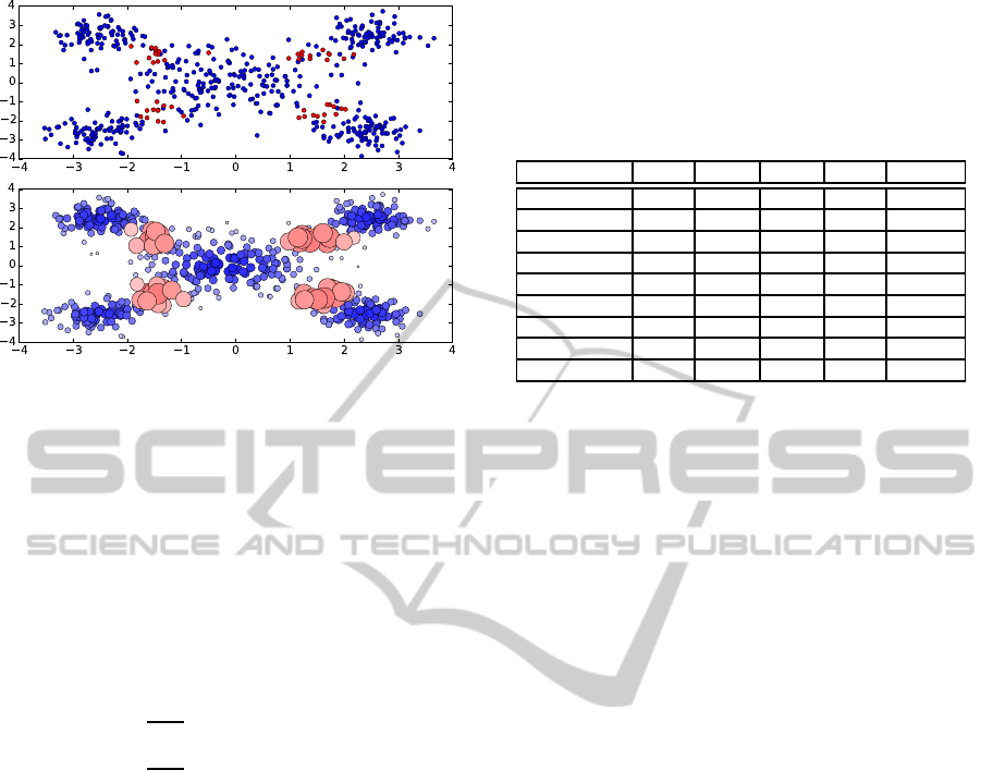
Figure 2: The distribution of examples (upper) and that of
fuzzy memberships (lower), that are associated to the exam-
ple weights given by the proposed method. The size of each
example and the deepness of its color express the magnitude
of the fuzzy membership associated to the example.
the kernel mean associated with a normalized PDS
kernel always exists.
In summary, we propose using a normalized char-
acteristic kernel k to calculate the example weight
f(x
i
) by the inner product of φ
φ
φ(x
i
) and ˆm
k
. More
precisely, we assign the example weights f(x
+
i
) and
f(x
−
i
) for the positive and negative examples, respec-
tively, as follows:
f(x
+
i
) =
1
kS
+
k
∑
(x
j
,y
j
)∈S
+
k(x
j
,x
+
i
),
f(x
−
i
) =
1
kS
−
k
∑
(x
j
,y
j
)∈S
−
k(x
j
,x
−
i
),
(7)
where S
+
ans S
−
are respective sets of the positive
and negative examples.
Remark that the proposed method enables the ex-
ample weight function to be multimodal, by consider-
ing the distribution of examples in the feature space.
In Figure 2, we show an instance of the relationship
between the distribution of the examples and the dis-
tribution of the fuzzy memberships. In the upper part,
50 positive examples (red) and 500 negative exam-
ples (blue) are drawn according to a distribution. In
the lower part, we illustrate the fuzzy memberships,
that are associated to the examples by our proposed
method. The size of each example and the deepness
of its color express the magnitude of the fuzzy mem-
bership associated to the example. As we see, the dis-
tribution of fuzzy memberships given by our method
is multimodal. Furthermore, the proposed method re-
quires no additional mechanism such as other internal
classifiers nor decaying functions, because it evalu-
ates each example weight directly by the inner prod-
uct of the empirical kernel mean and the image of the
example.
Table 1: The imbalanced datasets used in the experiments.
#Pos and #Neg represent the numbers of positive and neg-
ative examples, respectively, and Ratio = #Neg/#Pos. The
dimension of an input space is denoted by Dim. For multi-
class datasets, the class labeled PosLabel is selected as the
positive class and the other classes are regarded as the neg-
ative class.
Dataset #Pos #Neg Ratio Dim. PosLabel
Pima-Indian 268 500 1.9 8 1
Waveform 1657 3343 2.0 21 0
Haberman 81 225 2.8 3 2
Transfusion 178 570 3.2 4 1
Ecoli 77 259 3.4 7 2
Satimage 626 5809 9.3 36 4
Yeast 51 1433 28.1 8 5
Abalone 103 4074 39.6 7 15
Page-Block 115 5358 46.6 10 5
We now turn our attention to the computational
cost. As mentioned in Section 2.3, we need the Gram
matrix K = [k(x
i
,x
j
)]
ij
to solve the SVM optimization
problem in (4). Conversely, in our proposed method,
all example weights f(x
+
i
) and f (x
−
i
) in (7) can be
calculated easily from the Gram matrix alone and re-
quires no additional computations. Moreover, our
method requires neither decaying functions nor the
adjustment of additional parameters (see Figure 1).
Our method can be applied to any input space, if we
define a characteristic PDS kernel for it. Therefore,
our method is much more general than other methods.
4 EXPERIMENT
We compared the performance of our proposed
method with other learning methods, including the
original SVM, the DEC method, and six variations
of FSVM-CIL. We implemented these methods us-
ing the scikit-learn library (Pedregosa et al., 2011).
The
svm module works just as a wrapper of Lib-
SVM (Chang and Lin, 2011). The experiments are
performed on a 2.80GHz Intel
c
 Xeon CPU X5660
with 48GB RAM, running CentOS 6.2. We consid-
ered the nine benchmark class imbalanced datasets
from the UCI Machine Learning Repository (Bache
and Lichman, 2013) listed in Table 1. These datasets
are the same as (Batuwita and Palade, 2010), ex-
cept the one named “miRNA”, that had been consid-
ered since their previous work (Batuwita and Palade,
2009). We excluded it because it is not stored in UCI
Machine Repository.
To assess the methods, we used three measures:
the sensitivity (SE) measure, the specificity (SP) mea-
sure, and the geometric mean (GM). These measures
are commonly used in class imbalanced dataset ex-
periments (He and Ma, 2013; Batuwita and Palade,
ASimpleClassificationMethodforClassImbalancedDatausingtheKernelMean
331

Table 2: Classification results obtained for Pima-Indian, Waveform, Haberman, Transfusion, Ecoli and Satimage by the
proposed method, the six variations of FSVM-CIL, the DEC method, and the original SVM. We evaluated the sensitivity (SE),
specificity (SP), geometric mean (GM =
√
SE×SP), and calculation time (Time). Each value of SE, SP and GM is represented
as a percentage (%), and each one of Time is expressed in a second (sec).
Dataset Pima-Indian Waveform
method SE SP GM Time Rank SE SP GM Time Rank
proposed 71.6 77.8 74.7 0.14 1 90.8 85.5 88.1 7.79 5
FSVMCIL
cen
lin
67.1 78.4 72.5 0.31 2 91.7 85.6 88.6 2.72 1
FSVMCIL
sph
lin
62.2 62.4 62.3 0.91 7 93.5 83.8 88.5 22.86 2
FSVMCIL
hyp
lin
46.3 80.4 61.0 33326.54 9 75.9 96.2 85.4 195892.31 7
FSVMCIL
cen
exp
55.0 75.2 64.3 89.63 5 91.1 85.7 88.4 587.26 3
FSVMCIL
sph
exp
73.8 60.6 66.9 87.78 4 96.4 79.2 87.4 603.38 6
FSVMCIL
hyp
exp
45.2 86.0 62.3 32881.10 6 75.9 96.2 85.4 193904.45 8
SVM 53.4 85.8 67.7 - 3 83.5 93.0 88.1 - 4
DEC 42.6 88.2 61.3 0.03 8 75.7 96.2 85.3 0.02 8
Dataset Haberman Transfusion
method SE SP GM Time Rank SE SP GM Time Rank
proposed 61.5 70.7 65.9 0.04 2 54.6 54.3 54.5 0.17 2
FSVMCIL
cen
lin
61.5 73.8 67.3 0.18 1 50.7 58.1 54.3 0.24 3
FSVMCIL
sph
lin
45.6 63.1 53.6 0.21 6 60.3 35.2 46.1 0.79 8
FSVMCIL
hyp
lin
22.5 93.8 45.9 15747.52 8 18.2 88.3 40.1 55704.97 9
FSVMCIL
cen
exp
54.2 69.3 61.3 36.08 3 48.6 62.6 55.2 93.13 1
FSVMCIL
sph
exp
51.6 64.0 57.5 35.33 4 74.5 32.4 49.1 84.83 5
FSVMCIL
hyp
exp
24.4 77.8 43.6 15759.51 9 44.8 57.0 50.5 55795.26 4
SVM 41.8 78.7 57.4 - 5 23.9 89.4 46.2 - 7
DEC 29.3 74.2 46.7 0.02 7 25.4 87.6 47.2 0.01 6
Dataset Ecoli Satimage
method SE SP GM Time Rank SE SP GM Time Rank
proposed 83.6 85.9 84.8 0.02 2 86.1 84.3 85.2 19.00 3
FSVMCIL
cen
lin
83.6 84.4 84.0 0.13 4 87.4 83.6 85.5 4.97 2
FSVMCIL
sph
lin
84.5 81.6 83.0 0.28 7 90.4 81.9 86.1 39.28 1
FSVMCIL
hyp
lin
78.0 86.8 82.3 511.00 8 59.4 96.5 75.7 38066.44 7
FSVMCIL
cen
exp
82.3 85.2 83.7 42.03 5 83.1 76.6 79.7 723.25 4
FSVMCIL
sph
exp
89.5 77.3 83.2 38.4 6 74.9 77.8 76.4 818.29 5
FSVMCIL
hyp
exp
66.0 94.7 79.0 543.95 9 58.8 96.6 75.3 38658.07 9
SVM 84.3 84.0 84.2 - 3 59.9 96.1 75.8 - 6
DEC 90.0 83.2 86.5 0.00 1 59.2 96.4 75.6 0.04 8
2010; Akbani et al., 2004). The SE and SP measures
are the ratio of the correctly classified positive and
negative examples, respectively, to the total, and the
GM is given by GM =
√
SE×SP.
Through the experiments, we carried out the
outer-inner-cv (Batuwita and Palade, 2010), consist-
ing of two layers of five-fold cross validations. When
dividing a dataset into five partitions, we maintained
the ratio of the number of examples between positive
and negative classes because we are considering class
imbalanced datasets.
We used Gaussian kernels k
rbf
(x,x
′
) =
exp(−βkx − x
′
k
2
) (β > 0) in each classifier.
The Gaussian kernel is a popular kernel used in SVM
and has a characteristic property (Fukumizu et al.,
2013). For the inner-cv, we performed a two-step
search to obtain good values for the parameters
C in SVM and β in the Gaussian kernels. In the
first step, we performed a grid-parameter-search
for logC in the range {1,2, . . . , 15} and for logβ in
{−15, −14,..., −1} to obtain a roughly good pair
(
¯
C,
¯
β) of values. In the second step, we fine-tuned our
results through a grid-parameter-search for logC in a
narrower range log
¯
C ⊕{0,±0.25,±0.5,±0.75} and
for logβ in log
¯
β ⊕ {0,±0.25,±0.5, ±0.75}, where
v⊕S denotes the set {v+ s |s ∈ S}. We set δ = 10
−6
for the linearly decaying function in FSVM-CIL
according to the settings given by Batuwita and
Palade (2010). For the exponential decaying func-
tion, we selected ε from the range {0.1, 0.2,..., 1.0}
by adding a third axis to the grid-parameter-search.
Besides SE and SP, we show the total running time
KDIR2014-InternationalConferenceonKnowledgeDiscoveryandInformationRetrieval
332

Table 3: Classification results obtained for Yeast, Abalone, Page-block and the average of 9 datasets by the proposed method,
the six variations of FSVM-CIL, the DEC method, and the original SVM. We evaluated the sensitivity (SE), specificity (SP),
geometric mean (GM =
√
SE×SP), and calculation time (Time). Each value of SE, SP and GM is represented as a percent-
age (%), and each one of Time is expressed in a second (sec).
Dataset Yeast Abalone
method SE SP GM Time Rank SE SP GM Time Rank
proposed 84.2 85.2 84.7 1.27 1 73.3 68.1 70.6 8.06 2
FSVMCIL
cen
lin
80.4 85.9 83.1 0.48 3 73.3 66.7 69.9 1.46 3
FSVMCIL
sph
lin
57.3 80.0 67.7 2.63 5 72.5 54.0 62.6 15.4 4
FSVMCIL
hyp
lin
25.6 97.1 49.9 3140.44 8 67.6 32.2 46.6 64528.58 6
FSVMCIL
cen
exp
84.2 85.2 84.7 172.47 1 78.3 64.8 71.2 487.37 1
FSVMCIL
sph
exp
100.0 0.0 0.0 173.5 9 100.0 0.0 0.0 553.39 9
FSVMCIL
hyp
exp
64.0 58.1 61.0 3292.45 6 46.0 51.3 48.6 65907.74 5
SVM 82.4 80.6 81.5 - 4 88.6 17.3 39.1 - 8
DEC 36.5 94.4 58.7 0.03 7 69.6 30.0 45.7 0.07 7
Dataset Page-block average of 9 datasets
method SE SP GM Time Rank SE SP GM Time Rank
proposed 81.7 90.3 85.9 15.02 3 76.4 78.0 77.2 5.72 1
FSVMCIL
cen
lin
85.2 90.1 87.6 2.43 2 75.7 78.5 77.0 1.44 2
FSVMCIL
sph
lin
87.8 91.1 89.5 27.07 1 72.7 70.3 71.0 12.16 3
FSVMCIL
hyp
lin
37.4 94.7 59.5 6111.99 5 47.9 85.1 60.7 45892.20 8
FSVMCIL
cen
exp
0.0 100.0 0.0 692.91 9 64.1 78.3 65.4 324.90 5
FSVMCIL
sph
exp
45.2 66.0 54.6 693.08 6 78.4 50.8 52.8 343.11 9
FSVMCIL
hyp
exp
60.0 48.2 53.8 6804.82 7 53.9 74.0 62.2 45949.71 6
SVM 40.9 94.3 62.1 - 4 62.1 79.9 69.9 - 4
DEC 24.3 95.1 48.1 0.06 8 50.3 82.8 61.7 0.03 7
for evaluating example weights in each method, in
order to compare the actual computational costs
including parameter tuning. The time for computing
Gram matrix and solving the optimization problem
of SVM are excluded, because these are common to
all methods. More precisely, the running time refers
to the sum of the time for evaluating example weights
for all examples, that include parameter tuning in
outer-inner-cv.
The results are listed in Table 2 and 3. As shown,
our proposed method achieved the best performance
in the two datasets (Pima-Indian and Yeast) of the
nine datasets. Moreover, the proposed method got
high ranks in other datasets with various imbalance
ratios. Actually, our method performed the best on
the average of the nine GM measures. Concerning
with the running time, DEC and FSVMCIL
cen
lin
are
much faster than the other methods in all datasets.
This is because both DEC and FSVMCIL
cen
lin
runs in
O(n) time with respect to the number n of examples,
while the others require O(n
2
) time. Next to these
two methods, the proposed method runs fast, because
it does not depend on any other mechanisms, and
it has fewer parameters to adjust, among other
FSVIM-CIL methods. The FSVM-CIL methods
utilizing the exponential decaying function g
exp
are slow in general, because it takes time to adjust
the parameter ε for g
exp
. Obviously, FSVMCIL
hyp
lin
and FSVMCIL
hyp
exp
are much slower, because the
computation of d
hyp
S
(x
i
) requires another internal
SVM classifiers to execute.
5 CONCLUSION
We proposed a new method for the classification
problem associated with class imbalanced data. We
developed a simple but effective method to provide
a fuzzy membership for each example by consider-
ing the probability distribution over the feature space.
Our method reuses the Gram matrix, which is always
used in SVM, to obtain fuzzy membership values for
each example without additional computational cost.
Furthermore, our method does not rely on the ad-
justment of additional parameters. Experiments con-
firmed the superiority of our method over other clas-
sification methods for imbalanced data.
We note that our proposed method can be applied
also for non-vectorial data, such as strings, graphs,
and images, even though we do not have any charac-
teristic kernels for non-vectorial data yet. However, if
such characteristic kernels are developed, we can ap-
ply our method to non-vectorial data more effectively.
We will try to address them in future work.
ASimpleClassificationMethodforClassImbalancedDatausingtheKernelMean
333

REFERENCES
Akbani, R., Kwek, S., and Japkowicz, N. (2004). Applying
support vector machines to imbalanced datasets. In
Proc. of ECML, pages 39–50.
Bache, K. and Lichman, M. (2013). UCI machine learning
repository.
Batuwita, R. and Palade, V. (2009). micropred: effective
classification of pre-mirnas for human mirna gene pre-
diction. Bioinformatics, 25(8):989–995.
Batuwita, R. and Palade, V. (2010). FSVM-CIL: Fuzzy
support vector machines for class imbalance learning.
Trans. Fuz Sys., 18(3):558–571.
Bertinet, A. and Agnan, T. C. (2004). Reproducing Kernel
Hilbert Spaces in Probability and Statistics. Kluwer
Academic Publishers.
Burges, C. J. C. (1998). A tutorial on support vector ma-
chines for pattern recognition. Data Min. Knowl. Dis-
cov., 2(2):121–167.
Chang, C.-C. and Lin, C.-J. (2011). LIBSVM: A library
for support vector machines. ACM Transactions on
Intelligent Systems and Technology, 2:27:1–27:27.
Chun-Fu, L. and Sheng-De, W. (2002). Fuzzy support vec-
tor machines. IEEE Transactions on Neural Networks,
13(2):464–471.
Chun-Fu, L. and Sheng-De, W. (2004). Training algorithms
for fuzzy support vector machines with noisy data.
Pattern Recognition Letters, 25(14):1647–1656.
Cristianini, N., Kandola, J., Elisseeff, A., and Shawe-
Taylor, J. (2002). On kernel-target alignment. In Ad-
vances in NIPS 14, pages 367–373.
Duda, R. O. and Hart, P. E. (1973). Pattern Classification
and Scene Analysis. John Wiley & Sons Inc.
Fukumizu, K., Bach, F. R., and Jordan, M. I. (2009). Ker-
nel dimension reduction in regression. The Annals of
Statistics, 37(4):1871–1905.
Fukumizu, K., Song, L., and Gretton, A. (2013). Kernel
Bayes’ rule: Bayesian inference with positive defi-
nite kernels. Journal of Machine Learning Research,
14:3753–3783.
He, H. and Garcia, E. A. (2009). Learning from imbalanced
data. IEEE Transactions on Knowledge and Data En-
gineering, 21(9):1263–1284.
He, H. and Ma, Y. (2013). Imbalanced Learning: Foun-
dations, Algorithms, and Applications. Wiley-IEEE
Press, 1st edition.
Jiang, X., Yi, Z., and Lv, J. (2006). Fuzzy SVM with a
new fuzzy membership function. Neural Computing
& Applications, 15(3-4):268–276.
Mohri, M., Rostamizadeh, A., and Talwalkar, A. (2012).
Foundations of Machine Learning. The MIT Press.
Pedregosa, F., Varoquaux, G., Gramfort, A., Michel, V.,
Thirion, B., Grisel, O., Blondel, M., Prettenhofer,
P., Weiss, R., Dubourg, V., Vanderplas, J., Passos,
A., Cournapeau, D., Brucher, M., Perrot, M., and
Duchesnay, E. (2011). Scikit-learn: Machine learning
in Python. Journal of Machine Learning Research,
12:2825–2830.
Vapnik, V. N. (1995). The Nature of Statistical Learning
Theory. Springer-Verlag New York, Inc.
Veropoulos, K., Campbell, C., and Cristianini, N. (1999).
Controlling the sensitivity of support vector machines.
In Proc. of IJCAI, pages 55–60.
Yan, D., Liu, X., and Zou, L. (2013). Probability
fuzzy support vector machines. International Jour-
nal of Innovative Computing, Information and Con-
trol, 9(7):3053–3060.
KDIR2014-InternationalConferenceonKnowledgeDiscoveryandInformationRetrieval
334