
Evolutionary Optimization of a One-Class Classification System for
Faults Recognition in Smart Grids
Enrico De Santis
1
, Gianluca Distante
1
, Fabio Massimo Frattale Mascioli
1
, Alireza Sadeghian
2
and Antonello Rizzi
1
1
Dept. of Information Engineering, Electronics, and Telecommunications, “Sapienza” University of Rome,
Via Eudossiana 18, 00184 Rome, Italy
2
Dept. of Computer Science, Ryerson University, ON M5B 2K3, Toronto, Canada
Keywords:
Evolutionary Optimization, One Class Classification, Smart Grids, Fault Recognition.
Abstract:
The Computational Intelligence paradigm has proven to be a useful approach when facing problems related
to Smart Grids (SG). The modern SG systems are equipped with Smart Sensors scattered in the real-world
power distribution lines that are able to take a fine-grained picture of the actual power grid state gathering a
huge amount of heterogeneous data. Modeling and predicting general faults instances by means of processing
structured patterns of faults data coming from Smart Sensors is a very challenging task. This paper deals
with the problem of faults modeling and recognition on MV feeders in the real-world Smart Grid system that
feeds the city of Rome, Italy. The faults recognition problem is faced by means of a One-Class classifier
based on a modified k-means algorithm trained through an evolutive approach. Due to the nature of the
specific data-driven problem at hand, a custom weighted dissimilarity measure designed to cope with mixed
data type like numerical data, Time Series and categorical data is adopted. For the latter a Semantic Distance
(SD) is proposed, capable to grasp semantical information from clustered data. A genetic algorithm is in
charge to optimize system’s performance. Tests were performed on data gathered over three years by ACEA
Distribuzione S.p.A., the company that manages the power grid of Rome.
1 INTRODUCTION
The Smart Grid (SG) is one the best technologi-
cal breakthrough concerning efficient and sustainable
management of power grids. According to the defi-
nition of the Smart Grid European Technology Plat-
form a SG should “intelligently integrate the actions
of all the connected users, generators, consumers and
those that do both, in order to efficiently deliver sus-
tainable economic and secure electricity supply” (Eu-
ropean Technology Plat., 2013). To reach that global
goal the key word is the “integration” of technologies
and research fields to add value to the power grid.
The SG can be considered an evolution rather than
a “revolution” (Energy Information Admin., 2013)
with improvements in monitoring and control tasks,
in communications, in optimization, in self-healing
technologies and in the integration of the sustainable
energy generation. This evolution process is possible
if it will be reinforced by the symbiotic exchange with
Information Communications Technologies (ICTs),
that, with secure network technologies and powerful
computer systems, will provide the “nervous system”
and the “brain” of the actual power grid. Smart Sen-
sors are the fundamental driving technology that to-
gether with wired and wireless network communica-
tions and cloud systems are able to take a fine grained
picture not only of the power grid state but also of the
surrounding environment. At this level of abstraction,
the SG ecosystem act like a Complex System with an
inherent non-linear and time-varying behavior emerg-
ing from heterogeneous elements with high degree
of interaction, exchanging energy and information.
Computational Intelligence (CI) techniques can face
complex problems (Venayagamoorthy, 2011) and is a
natural way to “inject” intelligence in artificial com-
puting systems taking inspiration from the nature and
providing capabilities like monitoring, control, deci-
sion making and adaptations (De Santis et al., 2013).
An important key issue in SGs is the Decision
Support System (DSS), which is an expert system
that provides decision support for the commanding
95
De Santis E., Distante G., Mascioli F., Sadeghian A. and Rizzi A..
Evolutionary Optimization of a One-Class Classification System for Faults Recognition in Smart Grids.
DOI: 10.5220/0005124800950103
In Proceedings of the International Conference on Evolutionary Computation Theory and Applications (ECTA-2014), pages 95-103
ISBN: 978-989-758-052-9
Copyright
c
2014 SCITEPRESS (Science and Technology Publications, Lda.)

and dispatching system of the power grid. The in-
formation provided by the DSS can be used for Con-
dition Based Maintenance (CBM) in the power grid
(Raheja et al., 2006). Collecting heterogeneous mea-
surements in modern SG systems is of paramount im-
portance. As an instance, the available measurements
can be used for dealing with various important pattern
recognition and data mining problems on SGs, such as
event classification (Afzal and Pothamsetty, 2012), or
diagnostic systems for cables and accessories (Rizzi
et al., 2009). On the basis of the specific type of con-
sidered data, different problem types could be formu-
lated. In (Guikema et al., 2006) authors have estab-
lished a relationship between environmental features
and fault causes. A fault cause classifier based on
the linear discriminant analysis (LDA) is proposed in
(Cai and Chow, 2009). Information regarding weather
conditions, longitude-latitude information, and mea-
surements of physical quantities (e.g., currents and
voltages) related to the power grid have been taken
into account. The One-Class Quarter-Sphere SVM
algorithm is proposed (Shahid et al., 2012) for faults
classification in the power grid. The reported exper-
imental evaluation is however performed on synthet-
ically generated data only. This paper addresses this
topic, facing the challenging problem of faults predic-
tion and recognition on a real distribution network, in
order to report in real time possible defects, before
failures can occur, or as an off-line decision making
aid, within the corporate strategic management pro-
cedures. The data set provided by Acea Distribuzione
S.p.a (ACEA – the company managing the electrical
network feeding the whole province of Rome, Italy)
collects all the information considered by company’s
field experts as related to the events of a particular
type of faults, namely Localized Faults (LF). This
paper follows our previous work (De Santis et al.,
2014) where the posed problem of faults recognition
and prediction is framed as an unsupervised learning
problem approached with the One Class Classifica-
tion (OCC) paradigm (Khan and Madden, 2010) be-
cause of the availability only of positive or target in-
stances (faults patterns). This modeling problem can
be faced by synthesizing reasonable decision regions
relying on a k-means clustering procedure in which
the parameters of a suited dissimilarity measure and
the boundaries of decision regions are optimized by
a Genetic Algorithm, such that unseen target test pat-
terns are recognized properly as faults or not. This
paper focuses on two important issues: i) the initial-
ization of k-means with an automatic procedure in or-
der to find the optimal number k of clusters; ii) to find
a more reliable dissimilarity measure for the categor-
ical features of the faults patterns; to this aim, the Se-
mantic Distance (SD) is adopted, addressing the prob-
lem of better grasping the semantic content of a well-
formed cluster.
A brief review of the faults patterns is given in
Sect. 2.1, while in Sec. 2 will be introduced the
OCC system for fault recognition and the proposed
initialization procedure for the k-means algorithm. In
Sec. 2.4 is presented the weighted dissimilarity mea-
sure and the proposed SD for categorical features. In
Sec. ?? it is shown and discussed the experimental re-
sults in terms of classifications performances compar-
ing the well-known simple matching measure with the
proposed semantic distance for categorical attributes.
Finally, in the Sec. 4, conclusions are drawn.
2 THE ONE
CLASS-CLASSIFICATION
APPROACH FOR FAULTS
DETECTION
2.1 The Fault Patterns
The ACEA power grid is constituted of backbones of
uniform section exerting radially with the possibility
of counter-supply if a branch is out of order. Each
backbone of the power grid is supplied by two distinct
Primary Stations (PS) and each half-line is protected
against faults through the breakers. The underlined
SG is equipped with Secondary Stations (SSs) located
in the PSs able to collect faults data. A fault is related
to the failure of the electrical insulation (e.g., cables
insulation) that compromises the correct functioning
of (part of) the grid. Therefore, a LF is actually a fault
in which a physical element of the grid is permanently
damaged causing long outages. LFs must be distin-
guished from both: i) “short outages” that are brief
interruptions lasting more than one second and less
than three minutes; ii) “transient outages” in which
the interruptions don’t exceed one second. The last
ones can be caused, for example, by a transient fault
of a cable’s electrical insulation of very brief duration
not causing a blackout.
The proposed one-class classifier is trained and
tested on a dataset composed by 1180 LFs patterns
structured in 20 different features. The features be-
long to different data types: categorical (nominal),
quantitative (i.e., data belonging to a normed space)
and times series (TSs). The last ones describes the
sequence of short outages that are automatically reg-
istered by the protection systems as soon as they oc-
cur. LFs on MV feeders are characterized by hetero-
geneous data, including weather conditions, spatio-
ECTA2014-InternationalConferenceonEvolutionaryComputationTheoryandApplications
96

Table 1: Considered features representing a FP.
Feature Data type Description
(1) Day start Day in which the LF was detected.
(2) Time start Time stamp (minutes) in which the LF was detected.
(12) Current out of bounds Quantitative (Integer) The maximum operating current of the backbone is
less than or equal to 60% of the threshold “out of
bounds”, typically established at 90% of capacity.
(11) # Secondary Stations (SSs) Number of out of service secondary stations due to
the LF.
(3) Primary Station (PS) code Unique backbone identifier.
(4) Protection tripped Type of intervention of the protective device.
(5) Voltage line Categorical (String) Nominal voltage of the backbone.
(6) Type of element Element that caused the damage.
(17) Cable section Section of the cable, if applicable.
(7) Location element Element positioning (aerial or underground).
(8) Material Constituent material element (CU, AL).
(9) Primary station fault distance Distance between the primary station and the geo-
graphical location of the LF.
(10) Median point Fault location calculated as median point between
two secondary stations
(13) Max. temperature Maximum registered temperature.
(14) Min. temperature Minimum registered temperature.
(15) Delta temperature Quantitative (Real) Difference between the maximum and minimum
temperature.
(16) Rain Millimeters of rainfall in a period of 24 hours pre-
ceding the LF.
(18) Backbone Electric Current Extracted feature from Time Series of electric cur-
rent values that flows in a given backbone of the con-
sidered power grid. It is the difference between the
average of the current’s value, in two consecutive
temporal windows of twelve hours each one, before
the fault.
(18) Interruptions (breaker) Sequence of opening events of the breakers in the
primary station.
(19) Petersen alarms TS (Integers sequence) Sequence of alarms detected by the device called
“Petersen’s coil” due to loss of electrical insulation
on the power line.
(20) Saving interventions Sequences of decisive interventions of the Pe-
tersen’s coil which have prevented the LF.
temporal data (i.e., longitude-latitude pairs and time),
physical data related to the state of power grid and
its electric equipments (e.g., measured currents and
voltages), and finally meteorological data. The whole
database was provided by ACEA and contains data
concerning a temporal period of three years across
2009–2011. This database was validated, by cleaning
it from human errors and by completing in an appro-
priate way missing data. A detailed description of the
considered features is provided in Table 1.
2.2 The OCC Classifier
The main idea in order to build a model of LF pat-
terns in the considered SG is to use a clustering tech-
nique. In this work a modified version of k-means
is proposed, capable to find a suitable partitions P =
{C
1
,C
2
,...,C
k
} of data set and to determine at the
same time the optimal number of clusters k. The main
assumption is that similar status of the SG have sim-
ilar chances of generating a LF, reflecting the cluster
model. The OCC System is designed to find a proper
dicision region, namely the “faults space”, F , relying
on the positions of target patterns denoting the LFs. A
(one-class) classification problem instance is defined
as a triple of disjoint sets, namely training set (S
tr
),
validation set (S
vs
), and test set (S
ts
), all containing
FP instances. Given a specific parameters setting, a
classification model instance is synthesized on S
tr
and
it is validated on S
vs
. Finally, performance measures
are computed on S
ts
. As depicted in the functional
model (see Fig. 1) this paradigm is objectified by de-
signing the OCC classifier as the composition of three
modules wrapped in an optimization block. In order
to synthetize the LF region, the learning procedure is
leaded: 1) by the clustering module that operate an
hard partition of S
tr
; 2) by the validation module op-
erating on S
vs
, designed to refine the LF boundaries;
EvolutionaryOptimizationofaOne-ClassClassificationSystemforFaultsRecognitioninSmartGrids
97

Figure 1: Block diagram depicting the optimized classifica-
tion model synthesis.
Figure 2: Cluster decision region and its characterizing pa-
rameters.
the decision rule (that leads the task of the patterns
assignment) is based on the proximity of the LF pat-
tern at hand to the clusters representative. Thus the
core of the OCC system is the dissimilarity measure
d : F × F → R
+
, reported in Sec. 2.4, that depends
on a weighting parameter vector w. The decision re-
gions B(C
i
) are derived from a “cluster extent” mea-
sure δ(C
i
) characterizing the C
i
clusters and summed
to a tolerance parameter σ (thus B(C
i
)=δ(C
i
)+ σ) that
together to the dissimilarity weights belongs to the
search space for the optimization algorithm. Here C
i
is the i-th cluster (i = 1,2, ...,k) and δ(C
i
) is the aver-
age intra-cluster dissimilarity.
In this work in addition to the weights w and the
σ parameters the search space is completed by a γ pa-
rameter controlling the proposed k-means initializa-
tion algorithm (see Sec. 2.3). Finally it is defined the
search space, constituted by the all model’s parame-
ters, as p = [w, σ,γ].
In this work the representative of the cluster, de-
noted as c
i
= R(C
i
), is the MinSOD (Del Vescovo
et al., 2014). So for each cluster C
i
the representative
one will be chosen as the pattern that belongs to the
considered cluster and for which the sum of distances
from the other patterns of the cluster has the lower
value. A cluster representative c
i
can be considered as
a prototype of a typical fault scenario individuated in
S
tr
. The decision rule to establish if a test pattern is a
target pattern or not is performed computing its over-
all dissimilarity measure d from the representatives
of all clusters C
i
and verifying if it falls in the deci-
sion region (see Fig. 2) built up on the nearest cluster.
A standard Genetic Algorithm is used in the learn-
ing phase in order to minimize the trade-off between
the classification error rate on S
vs
and the threshold σ
0
Figure 3: Composition of the chromosome.
value by means of the following Objective Function:
f (p) = α ER(S
vs
) + (1 − α) σ
0
, (1)
where α ∈ [0,1] is an external parameter controlling
the importance in minimizing ER(S
vs
) versus σ
0
. In
other words, α is a meta-parameter by which it is
possible to control the relative importance in mini-
mizing th error rate on S
vs
or in minimizing the over-
all faults decision region extent. σ
0
is the threshold
value normalized with respect to the diagonal D of
the hypercube (see Sec. 2.4 ) of the overall space:
σ
0
= σ/D. As concerns the chromosome coding (see
Fig. 3), each individual of the population consists in
the weights w
s
, s = (1,2,...,N
w
) associated to each
feature, where N
w
is the number of the considered fea-
tures, the value σ that is the threshold added at each
“cluster extent” measure during the validation phase
and the γ parameter mentioned above. The overall
number of genes in an individual’s chromosome is
therefore l=N
w
+ 2. The functional dependencies be-
tween the discussed parameters, in the proposed OCC
system, are:
k
opt
= k
opt
(w,γ)
σ
i
= σ
i
(k
opt
,w)
RR = RR(w,σ
i
),
(2)
where k
opt
is the optimum number of clusters found
by the k-means initialization algorithm described in
the next Sec. and RR = 1 − ER is the Recognition
Rate of the proposed (one-class) classifier. The sub-
script index i covers the general case, not studied here,
in which can be instantiated distinct thresholds values
for different clusters.
2.3 The k-means Initialization
Algorithm
It is well known that the k-means behaviour depends
critically on both the number k of clusters, given
as a fixed input, and on the position of the k initial
clusters representatives. In the literature there are a
wide range of algorithms for the initialization of the
centroids of the k-means, each with its pros and cons
(Dan Pelleg, 2000; Tibshirani et al., 2001; Laszlo
and Mukherjee, 2006). The initialization criterion
of centroids, here proposed, was initial inspired by
(Barakbah and Kiyoki, 2009). The work is based on
the idea to choose as centroids, the patterns that are
furthest from each other. The provided version of
ECTA2014-InternationalConferenceonEvolutionaryComputationTheoryandApplications
98

the algorithm takes into account also the presences
of outliers. To verify if the candidate centroid is an
outlier we designed a simple decision rule defined by
parameters: a, an integer value, and b, a real valued
number ranging [0,1]. The parameter a indicates the
minimum number of patterns that must enter in the
circumference with center the pattern candidate as
centroid and radius given by b ∗ d
Pmax
, where d
Pmax
is
the distance between the furthest pattern in the whole
dataset. Hence if within the distance b ∗ d
Pmax
there
are more than a patterns then the candidate centroid
is not an outlier. Other inputs to the overall algorithm
are a scale parameter γ, the dissimilarity matrix D and
the number of initially centroid k
ini
. The algorithm
tries to calculate the best positions of the centroids
and their final number k
opt
possibly decreasing the
provided initial number (k
ini
). The main steps are the
following:
Algorithm input: The initial number of centroids k
ini
, the
dissimilarity matrix D, the γ ∈ [0,1] parameter, a,b, d
Pmax
.
Algorithm output: the k
opt
centroids.
Choose a random pattern p
i
among those available in
S
tr
and compute the pattern p
j
furthest away from it.
while centroid==not found do
if p
j
is not an outlier then
choose p
j
as the first centroid;
centroid=found;
else
choose as p
j
the next pattern among those fur-
thest away from p
i
;
centroid=not found;
end
end
Choose as second centroid the pattern p
a
furthest away
from p
j
.
while centroid==not found do
if p
a
is not an outlier then
choose it as the as second centroid;
centroid=found;
else
choose as p
a
the next pattern furthest away
from p
j
;
centroid=not found
end
end
while k < k
ini
do
choose as a possible centroid the pattern p
n
whose
sum of the distances to the other centroids, found ear-
lier, is maximum;
if p
n
is not an outlier then
choose it as the other centroid; k = k + 1;
else
choose the next pattern whose sum of the dis-
tances to the other centroids found earlier, is max-
imum;
end
end
Calculate d
Cmax
= d(p
j
, p
a
) as the distance between the
first two centroids. Given the external parameter γ ∈ [0, 1]
for i=1; i < k; i++ do
for j=1; j < k; j++ do
if d(p
i
, p
j
) ≤ γ ∗ d
Cmax
then
delete randomly one of the two considered
centroid, k = k
ini
− 1;
end
end
end
return the k
opt
= k centroids.
The k-means with the proposed representatives
initialization can be seen as an hybrid between a k-
clustering and a free clustering algorithm where, once
fixed an initial number of centroids, it returns an op-
timal number of centroids less or equal to the initial
ones.
2.4 The Weighted Custom Dissimilarity
Measure
The dissimilarity function between two patterns is of
paramount importance in data driven modeling appli-
cations. Given two patterns x and y the wighted dis-
similarity measure adopted in the proposed classifier
is:
d(x,y;W ) =
q
(x y)WW
T
(x y)
T
) (3)
d(x,y;W ) ∈ [0,D]
where (x y) is a Component-Wise dissimilarity
measure, i.e. a row vector containing the specific
differences between homologues features. W is
a diagonal square matrix of dimension N
w
× N
w
,
in which N
w
is the number of weights. In Eq. 3
the maximum value for d is the diagonal of the
hypercube, that is: D =
q
∑
N
w
i=1
w
2
i
, where w
i
are the
features weights. The inner specific dissimilaritiy
functions differ each other depending on the nature
of each feature as explained in the following.
Quantitative (real). Given two normalized quanti-
tative values v
i
,v
j
the distance between them is the
absolute difference: d
i, j
=| v
i
− v
j
|.
As regards the features “Day start” and “Time
start” the distance is calculated through the circular
difference. The value of these features is an integer
number between 1 and 365 (total days in one year)
for the former and between 1 and 1140 (total minutes
in one day) for the latter. The circular distance be-
tween two numbers is defined as the minimum value
between the calculated distance in a clockwise direc-
tion and the other calculated in counter clockwise.
Categorical (nominal). Categorical attributes, also
referred to as nominal attributes, are attributes with-
out a semantically valid ordering (see Tab. 1 for the
EvolutionaryOptimizationofaOne-ClassClassificationSystemforFaultsRecognitioninSmartGrids
99

Figure 4: Sketch of circular domains for “Day start” and
“Time start” features.
data treated as nominal). Let’s define c
i
and c
j
the val-
ues of the categorical feature for the patterns i-th and
j-th, respectively. A one well-suited solution to com-
pute a dissimilarity measure for categorical features is
the Simple-Matching (SM) distance:
d
i, j
=
(
1 i f c
i
6= c
j
0 i f c
i
= c
j
.
(4)
When measuring pattern-cluster dissimilarities (i.
e. in the assignment of a pattern to a clusters) the Se-
mantic Distance (SD) introduced in Sec. 2.4.1 is used.
Times Series TSs are characterized by a non-uniform
sampling since they represent sequences of asyn-
chronous events. As a consequence, usually they
don’t share the same length. TSs are represented
as real valued vectors containing the differences be-
tween short outages timestamps and the LF timestamp
considered as a common reference. These values are
normalized in the range [0, 1], dividing the values ob-
tained by the total number of seconds in the tempo-
ral window considered. In order to measure the dis-
tance between two different TSs (different in values
and size), we use the Dynamic Time Warping (DTW)
(M
¨
uller, 2007).
2.4.1 Semantic Distance for Categorical Data
The task of calculating a good similarity measure be-
tween categorical objects is challenging because of
the difficulties to establish meaningful relations be-
tween them. The distance between two objects com-
puted with the simple matching similarity measure
(Eq. 4) is either 0 or 1. This often results in clus-
ters with weak intra-similarity (Ng et al., 2007) and
this may result in a loss of semantic content in a par-
tition generated by a clustering algorithm. As con-
cerns k-modes (Huang, 1998) algorithm, in the liter-
ature several frequency-based dissimilarity measures
between categorical object are proposed (Cheng et al.,
2004; Quang and Bao, 2004). The proposed dissimi-
larity measure for categorical objects is a frequency-
based dissimilarity measure and follows the work (He
et al., 2011) in which a features weighted k-modes al-
gorithm is studied, where the weights are related to
the frequency value of a category in a given cluster.
Let N
i, j
be the number of instances of the i-
th value of the considered categorical feature F
cc
in the cluster j-th (C
j
) and let’s define N
max, j
=
max(N
1, j
,...N
n, j
), where n is the number of the differ-
ent values of F
cc
present in C
j
. We can finally define
the SD between a categorical feature of the pattern P
h
(F
cc
P
h
) and the cluster C
j
as:
d
F
cc
P
h
,C
j
= 1 −W
i, j
, with d
F
cc
P
h
,C
j
∈ [0, 1] (5)
where W
i, j
=
N
i, j
N
max, j
is the fraction of values of the i-th
category of the considered categorical feature in the
j-th cluster with respect to the number of values of
the most frequent category.
The SD take into account the statistical information of
a given cluster and it is used like a pattern-cluster dis-
similarity measure. Unlike the SM distance, the SD
can span in the real valued range [0, 1]. Note that this
distance is characterized by the statistical properties
of the specific cluster under consideration. The SD
can be intended as a “local metric”, since each cluster
is characterized by its own statistic distribution of cat-
egorical values and thus it is characterized by its own
weights that can change from one cluster to another.
For example, let us consider a categorical feature
coding for one of four possible colors (red, green,
blue or yellow) and let us consider the cluster
depicted in Fig 5. By means of Eq. (5) it is possible
Figure 5: In this cluster the Yellow feature value is com-
pletely missing.
to compute the values of W
i,L
for each color (nominal
attribute value), represented or not in the considered
cluster and then the SD:
(
W
R,L
=
10
10
,W
G,L
=
3
10
,W
B,L
=
5
10
i f Color 3 C
L
=> W
Color,L
= 0
• if the value of F
cc
P
h
is red: d
F
cc
P
h
,C
L
= 1 −
10
10
= 0
• if the value ofF
cc
P
h
is green: d
F
cc
P
h
,C
L
= 1 −
3
10
=
7
10
• if the value of F
cc
P
h
is blue: d
F
cc
P
h
,C
L
= 1 −
5
10
=
1
2
• if the value of F
cc
P
h
is yellow: d
F
cc
P
h
,C
L
= 1 −
0
10
= 1
ECTA2014-InternationalConferenceonEvolutionaryComputationTheoryandApplications
100
3 EXPERIMENTAL RESULTS
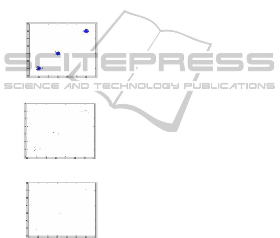
3.1 Test on k-means Initialization
Algorithm
The proposed initialization algorithm has been tested
on a toy problem, where patterns are generated from
three distinct Gaussian distributions, as depicted in
Fig. 6. Setting the initial number of centroids K
ini
=10,
the proposed algorithm converges to an optimal num-
ber of clusters equal to 3 (see also Fig. 7).
Figure 6: Patterns distribution in the considered toy prob-
lem.
(a) Centroids found before the close
representatives removal step, with
k
ini
= 10.
(b) The final optimal centroids
(K
opt
= 3).
Figure 7
3.2 Tests on ACEA Dataset
In this section we report the first tests of the proposed
OCC system on real data. The synthetized classifica-
tion model should be able to correctly recognize fault
patterns and, at the same time, to avoid raising wrong
alarm signals, recognizing as faults system’s measure-
ments corresponding to normal operating conditions.
Since non-faults patterns (negative instances) are not
available in the ACEA dataset, in order to properly
measure system performances, two distinct test sets
have been employed. The first one, namely Ts1, is a
subset of the available data set, i.e. a set of patterns
labeled as faults. Obviously, the classification accu-
racy on this test set should be as high as possible. As
concerns avoiding false positive misclassifications, a
second test set, namely Ts2, has been created as a uni-
form random sampling of the whole input space do-
main, introducing constraints related to the physical
network and environmental conditions in which the
SG is located; thus Ts2 contains patterns labelled as
both faults and non-faults. A high classification ac-
curacy on Ts2 must be interpreted as a clue of a high
number of false alarms, due to a too wide fault deci-
sion region. In close cooperation with the Acea ex-
perts, following their precious advice the LF model is
trained on the features 1 to 4 and 6 to 18 (described in
Tab. 1). Eighteen simulations, differing in the setting
of α=[0.3, 0.5, 0.7] parameter and of k
ini
= [15,10, 7]
parameter, have been carried out, adopting both the
proposed SD and the SM as pattern to clusters dis-
similarity measure for categorical feature subspaces,
yielding two different classification models, namely
A and B, respectively. Best results are reported in
Tab. 2. Although model B is characterized by a higher
classification accuracy on faults patterns (Ts1), model
A performs much better on Ts2 (the lower the better,
when performance on Ts1 are comparable), since its
fault decision region characterize much better faults
pattern, with a much more limited extension in the
whole input domain, avoiding thus to cover non-faults
pattern. To confirm this interpretation we have com-
puted the Davies-Bouldin index (Davies and Bouldin,
1979) on the training set partitions corresponding to
models A and B. The Davies-Bouldin index (DB in
Tab. 2) is a relative measure of compactness and
separability of clusters (the lower the better). These
measures confirm that clusters underlying the classi-
fication model A are more compact, yielding a much
more effective and essential faults decision region.
These results show that the proposed SD is much
more suited in defining an effective inductive infer-
ence engine when dealing with categorical features
subspaces, with respect to the plain SM distance.
4 CONCLUSIONS
In this paper we propose a MV lines faults recogni-
tion system as the core element of a Condition Based
EvolutionaryOptimizationofaOne-ClassClassificationSystemforFaultsRecognitioninSmartGrids
101

Table 2: Result of the best simulation obtained with the SD and SM.
Model α
f
k
i
k
opt
Categorical distance γ % Ts1 % Ts2 DB
A 0.3 7 7 Semantic Dissimilarity (SD) 0.4033 91.46% 23,12% 8.86
B 0.3 7 7 Simple Matching (SM) 0.4181 98,78% 35.76% 15.4
Maintenance procedure to be employed in the elec-
tric energy distribution network of Rome, Italy, man-
aged by ACEA Distribuzione S.p.A. By relying on
the OCC approach, the faults decision region is syn-
thetized by partitioning the available samples of the
training set. A suited pattern dissimilarity measure
has been defined in order to deal with different fea-
tures data types. The adopted clustering procedure
is a modifed version of k-means, with a novel proce-
dure for centroids initialization. A genetic algorithm
is in charge to find the optimal value of the dissimilar-
ity measure weights, as well as two parameters con-
trolling the initial centroids positioning and the fault
decision region extent, respectively. According to our
tests, the new proposed method for k-means initializa-
tion shows a good reliability in finding automatically
the best number of clusters and the best positions of
the centroids. Furthermore, the proposed SD for cat-
egorical features subspaces performs better than the
plain SM distance when used to define a pattern to
cluster dissimilarity measure. Since faults decision
region is synthetized starting from each cluster de-
cision region, this measure has a key role in defin-
ing a proper inductive inference engine, and thus in
improving the generalization capability of the recog-
nition system. Future works will be focused on the
definition of a suitable reliability classification mea-
sure, computed as the membership of incoming mea-
sures (patterns) to the fault decision region. Lastly,
tests results performed on real data make us confi-
dent about further systems developments possibility,
towards a final commissioning into the Rome electric
energy distribution network.
ACKNOWLEDGEMENTS
The authors wish to thank Acea Distribuzione S.p.A.
for providing the faults data and for their useful sup-
port during the OCC system design and test phases.
Special thanks to Ing. Stefano Liotta, Chief Network
Operation Division, and to Ing. Silvio Alessandroni,
Chief Electric Power Distribution Remote Control Di-
vision.
REFERENCES
Afzal, M. and Pothamsetty, V. (2012). Analytics for dis-
tributed smart grid sensing. In Innovative Smart Grid
Technologies (ISGT), 2012 IEEE PES, pages 1–7.
Barakbah, A. and Kiyoki, Y. (2009). A pillar algorithm for
k-means optimization by distance maximization for
initial centroid designation. pages 61–68.
Cai, Y. and Chow, M.-Y. (2009). Exploratory analysis of
massive data for distribution fault diagnosis in smart
grids. In Power Energy Society General Meeting,
2009. PES ’09. IEEE, pages 1–6.
Cheng, V., Li, C.-H., Kwok, J. T., and Li, C.-K. (2004). Dis-
similarity learning for nominal data. Pattern Recogni-
tion, 37(7):1471 – 1477.
Dan Pelleg, A. M. (2000). X-means: Extending k-means
with efficient estimation of the number of clusters. In
Proceedings of the Seventeenth International Confer-
ence on Machine Learning, pages 727–734, San Fran-
cisco. Morgan Kaufmann.
Davies, D. L. and Bouldin, D. W. (1979). A cluster separa-
tion measure. IEEE Transactions on Pattern Analysis
and Machine Intelligence, PAMI-1(2):224–227.
De Santis, E., Rizzi, A., Livi, L., Sadeghian, A., and Frat-
tale Mascioli, F. M. (2014). Fault recognition in smart
grids by a one-class classification approach. In 2014
IEEE World Congress on Computational Intelligence.
IEEE.
De Santis, E., Rizzi, A., Sadeghian, A., and Frattale Mas-
cioli, F. M. (2013). Genetic optimization of a fuzzy
control system for energy flow management in micro-
grids. In 2013 Joint IFSA World Congress and
NAFIPS Annual Meeting, pages 418–423. IEEE.
Del Vescovo, G., Livi, L., Frattale Mascioli, F. M., and
Rizzi, A. (2014). On the Problem of Modeling Struc-
tured Data with the MinSOD Representative. Interna-
tional Journal of Computer Theory and Engineering,
6(1):9–14.
Energy Information Admin. (2013). International Energy
Outlook 2011 - Energy Information Administration,
note=http://www.eia.gov/forecasts/ieo/index.cfm.
European Technology Plat. (2013). The Smart-
Grids European Technology Platform,
note=http://www.smartgrids.eu/ETPSmartGrids.
Guikema, S. D., Davidson, R. A., and Haibin, L. (2006).
Statistical models of the effects of tree trimming on
power system outages. IEEE Transactions on Power
Delivery, 21(3):1549–1557.
He, Z., Xu, X., and Deng, S. (2011). Attribute value weight-
ing in k-modes clustering. Expert Systems with Appli-
cations, 38(12):15365 – 15369.
Huang, Z. (1998). Extensions to the k-means algorithm for
clustering large data sets with categorical values.
ECTA2014-InternationalConferenceonEvolutionaryComputationTheoryandApplications
102

Khan, S. S. and Madden, M. G. (2010). A survey of recent
trends in one class classification. In Coyle, L. and
Freyne, J., editors, Artificial Intelligence and Cogni-
tive Science, volume 6206 of Lecture Notes in Com-
puter Science, pages 188–197. Springer Berlin Hei-
delberg.
Laszlo, M. and Mukherjee, S. (2006). A genetic algorithm
using hyper-quadtrees for low-dimensional k-means
clustering. Pattern Analysis and Machine Intelligence,
IEEE Transactions on, 28(4):533–543.
M
¨
uller, M. (2007). Dynamic time warping. In Informa-
tion Retrieval for Music and Motion, pages 69–84.
Springer Berlin Heidelberg.
Ng, M. K., Junjie, M., Joshua, L., Huang, Z., and He, Z.
(2007). On the impact of dissimilarity measure in k-
modes clustering algorithm. IEEE Transactions on
Pattern Analysis and Machine Intelligence.
Quang, L. and Bao, H. (2004). A conditional probability
distribution-based dissimilarity measure for categorial
data. In Dai, H., Srikant, R., and Zhang, C., editors,
Advances in Knowledge Discovery and Data Mining,
volume 3056 of Lecture Notes in Computer Science,
pages 580–589. Springer Berlin Heidelberg.
Raheja, D., Llinas, J., Nagi, R., and Romanowski, C.
(2006). Data fusion/data mining-based architecture
for condition-based maintenance. International Jour-
nal of Production Research, 44(14):2869–2887.
Rizzi, A., Mascioli, F. M. F., Baldini, F., Mazzetti, C., and
Bartnikas, R. (2009). Genetic optimization of a PD
diagnostic system for cable accessories. IEEE Trans-
actions on Power Delivery, 24(3):1728–1738.
Shahid, N., Aleem, S., Naqvi, I., and Zaffar, N. (2012). Sup-
port vector machine based fault detection amp; classi-
fication in smart grids. In Globecom Workshops (GC
Wkshps), 2012 IEEE, pages 1526–1531.
Tibshirani, R., Walther, G., and Hastie, T. (2001). Estimat-
ing the number of clusters in a data set via the gap
statistic. Journal of the Royal Statistical Society: Se-
ries B (Statistical Methodology), 63(2):411–423.
Venayagamoorthy, G. K. (2011). Dynamic, stochastic, com-
putational, and scalable technologies for smart grids.
IEEE Computational Intelligence Magazine, 6(3):22–
35.
EvolutionaryOptimizationofaOne-ClassClassificationSystemforFaultsRecognitioninSmartGrids
103
