
Joint Stiffness Identification of a Heavy Kuka Robot with a Low-cost
Clamped End-effector Procedure
A. Jubien
1,2
, G. Abba
3
and M. Gautier
1
1
IRCCyN (Institut de Recherche en Communications et Cybernétique de Nantes), Nantes, France
2
ONERA (The French Aerospace Lab), Toulouse, France
3
Dep. of Design, Manufacturing and Control (LCFC) and ENIM (National College of Engineering of Metz), Metz, France
Keywords: Stiffness, Industrial, Robot, Identification, Clamped End-effector.
Abstract: This paper proposes two new methods for the identification of static stiffnesses of multi degrees of freedom
heavy industrial robots. They are based on a locked link joint procedure obtained with an end-effector fixed
to the environment. The first method requires only measurements of motor positions and motor torques data
computed from motor current measurements and manufacturer's drive gains. The second one needs a torque
sensor to measure the interaction wrench between the clamped end-effector and the environment. These
methods are being experimentally validated and compared on the 2 first joints of a 6 degrees of freedom
heavy 500Kg payload industrial Kuka KR500 robot.
1 INTRODUCTION
New applications of heavy industrial robots for
performing machining operations like Friction Stir
Welding process (FSW) need trajectories with a high
accuracy end-effector position while significant
forces are applied to the end-effector.
It is then necessary to identify accurately the
stiffnesses to control and simulate precise and
reliable motion. Identification of rigid robots has
been widely investigated in the last decades, based
on the Inverse Dynamic Identification Model and
Least Squares estimation (IDIM-LS) (Hollerbach et
al., 2008). Several approaches can be used to
identify the dynamic parameters and joint dynamic
stiffnesses. One approach is based on IDIM-LS
technique and needs motor and joint positions and
motor torques (Pham et al., 2001); (Janot et al.,
2011). However, the joint positions are not measured
on industrial robots. Another approach is a closed-
loop output error method which needs to simulate
the robot (Gautier et al., 2013); (Östring, 2003).
Unfortunately, manufacturers do not want to give
the control laws of their controllers.
Another approach avoids using any internal data
(joint position, motor torque, control law) but it
requires an external measurement of the position of
the end-effector using very expensive laser-tracker
sensor with variation of the payload while the motor
positions are locked to constant values (Dumas et
al., 2011); (Alici and Shirinzadeh, 2005). In (Pfeiffer
and Holzl, 1995), each robot links are fixed
alternately to identify the current joint stiffness with
quasi-static test but this requires a different locking
system for each link.
To overcome theses expensive and heavy
procedures, this paper proposes two new methods
based on a locked link joint procedure obtained with
the end-effector clamped to the environment. The
first method requires only motor positions
measurement and motor torques data calculated
from motor current measurement and manufacturer's
drive gain data. The second one needs a torque
sensor to measure the external interaction wrench
between the clamped end-effector and the
environment, which are calculated as external link
torques using the jacobian matrix of the robot. A
first validation of our methodologies are carried out
on the 2 first joints of a 6 Degrees of Freedom (dof)
heavy 500Kg payload industrial Kuka KR500 robot.
This paper is divided into 5 sections. Section 2
describes the modeling of serial robots with the end-
effector attached to the base. Section 3 presents the
usual method for dynamic identification of robots,
based on IDIM-LS method. Section 4 is devoted to
the modeling of the Kuka KR500 heavy industrial
robot and to the identification of the first two axis of
the robot. The last section gives the conclusion.
585
Jubien A., Abba G. and Gautier M..
Joint Stiffness Identification of a Heavy Kuka Robot with a Low-cost Clamped End-effector Procedure.
DOI: 10.5220/0005115805850591
In Proceedings of the 11th International Conference on Informatics in Control, Automation and Robotics (ICINCO-2014), pages 585-591
ISBN: 978-989-758-040-6
Copyright
c
2014 SCITEPRESS (Science and Technology Publications, Lda.)

2 MODELING
2.1 Inverse Dynamic Identification
Model with Fixed End-effector
The Inverse Dynamic Model (IDM) of a flexible
robot calculates the motor torques and joint torques
as a function the joint and motor positions. It can be
obtained from the Newton-Euler or the Lagrangian
equations (Khalil and Dombre, 2002). It is given by
the following relation with no constraint applied on
the end-effector when the positions are quasi-
constants (no frictions and inertias effects):
_
_
_
()
()
()
idm m m
T
idm l e
idm l m
k q q Offm
Gq J q F
kq q
(1)
where
m
q ,
m
q
and
m
q
are respectively the (nx1)
vectors of motor positions, velocities and
accelerations;
q is the (nx1) joint position; τ
idm_m
is
the (nx1) vector of motor torques; τ
idm_l
is the (nx1)
vector of joint torque; k is the (nxn) diagonal matrix
of stiffness parameters; G(q) is the (nx1) vector of
gravity torque; Offm is the (nx1) vector of motor
current amplifier offset parameters; n is the number
of moving links. All measurement and mechanical
variables are given in S.I. unit in joint side.
J
T
(q) is the transpose of the jacobian matrix of
the robot and F
e
is the interaction wrench between
the end-effector and the base:
T
e
exyzxyz
e
f
Ffffmmm
m
(2)
The interaction force f
e
is composed of the three
forces f
x
, f
y
and f
z
; and the interaction moment m
e
is
composed of the three moment m
x
, m
y
and m
z
.
For a 6 dof robot with rigid links and with the
end-effector fixed to the environment, the joint link
position vector keep a constant value
00m
qq
,
where
0m
q is the motor position measured when the
motor torques and the interaction wrench are close
to zero. Then in the following, the jacobian matrix is
calculated with
0m
q :
00m
J
qJq Jq
(3)
The equations (1) becomes:
_0
_00
_0
()
()
()
idm m m
T
idm l e
idm l m
k q q Offm
Gq J q F
kq q
(4)
Introducing two offset parameters offkm and offkl,
the previous equation becomes:
_
0
_0
_
00
with
with ( )
idm m m
T
idm l e
idm l m
k q offkm
offkm offm k q
Jq F
k q offkl
offkl k q G q
(5)
The proposed model take into account only the joint
stiffness. However the link stiffness are unknown.
But, in practice, the stiffness identified values with
our model are the addition of the actual joint
stiffnesses and a part of link stiffnesses.
Accordingly, the identified model is accurate with
respect of the deformations of the robot.
2.2 Inverse Dynamic Identification
Model for Joint Stiffness
Identification with Motor Torques
Here, we especially want to identify the joint
stiffness. Writing (5) for axis j, the motor torque is
function of the joint stiffness of axis j:
_
idm m j j mj j
kq offkm
(6)
The motor torque of joint j can be expressed linearly
in relation to the set of dynamic parameters χ
stm j
(Gautier and Khalil, 1990) to get the IDIM:
_
idm m j stm j m stm j
IDM q χ
(7)
Where
s
tj m
I
DM q is the (1xNs) Jacobian matrix
of τ
idm_m j
, with respect to the (Nsx1) vector χ
stm j
of
the parameters.
χ
stm j
is composed of parameters of axis j with
fixed end-effector:
_
1
with
idm m j mj stm j
T
stm j j j
q χ
χ k Offkm
(8)
The motor torque τ
m j
is computed from the a priori
joint drive gain
ap
j
g
given by manufacturer's data
and the motor current I
j
for each axis j:
ap
mj j j
gI
(9)
ICINCO2014-11thInternationalConferenceonInformaticsinControl,AutomationandRobotics
586

2.3 Inverse Dynamic Identification
Model for Joint Stiffness
Identification with External
Wrench
Writing (4) for axis j, the external torque of axis j is
function of the joint stiffness of axis j:
_idm l j j m j j
k q offkl
(10)
The joint torque of joint j can be expressed linearly
in relation to joint stiffness and offset parameters χ
stl
j
:
_
1
with
idm l j mj
T
stl j j j
q
χ
k Offkl
(11)
The external torques τ
l
can be calculated from the
interaction wrench and the jacobian matrix (3) of the
robot (Khalil and Dombre, 2002):
0
T
le
J
qF
(12)
It is necessary to have good condition number for
the jacobian matrix to have a good estimation of the
joint torque.
3 IDIM-LS: INVERSE DYNAMIC
IDENTIFICATION MODEL
WITH LEAST SQUARES
METHOD
Because of perturbations due to noise measurement
and modeling errors, the actual torque
differs
from τ
idm
by an error e , such that:
idm m
eIDMq
χ
e
(13)
The vector
χ
ˆ
is the least squares (LS) solution of an
over determined system built from the sampling of
(13), while the elastic deformations vary on the
robot:
YW
(14)
Where:
Y is the (x1)r measurement vector, W the
(x)rbobservation matrix, and
is the (x1)r vector
of errors. The number of rows is r=nxn
e
, where the
number of recorded samples is n
e
.
Standard deviations
i
ˆ
, are estimated assuming
that
W is a deterministic matrix and
, is a zero-
mean additive independent Gaussian noise, with a
covariance matrix
T2
()
r
CE
ρ
ρ I
(Gautier,
1997); (Janot et al., 2014).
Where E is the expectation operator and I
r
, the
(rxr) identity matrix. An unbiased estimation of the
standard deviation
is the following:
2
2
()
ˆ
ˆ
Y-W r b
(15)
The covariance matrix of the estimation error is
given by:
T2T1
[( )( ) ] ( )
ˆˆ
ˆ
ˆˆ
CEχχχχ WW
(16)
The relative standard deviation
ri
ˆ
%
is given by:
100 , for
ri i
ˆˆ
ii
ˆˆ
%0
(17)
Where
()
i
2
ˆˆˆ
Ci,i
is the i
th
diagonal coefficient
of
ˆˆ
C
. Calculating the LS solution of (14) from
perturbed data in
W and Y may lead to bias if W
is correlated to
. Then, it is essential to filter data
in
Y and W before computing the LS solution.
Velocities and accelerations are estimated by means
of a band-pass filtering of the positions. To eliminate
high frequency noises and torque ripples, a parallel
decimation is performed on
Y and on each column
of
W . More details about data filtering can be
found in (Gautier, 1997) and (Pham et al., 2001).
4 EXPERIMENTAL
VALIDATION
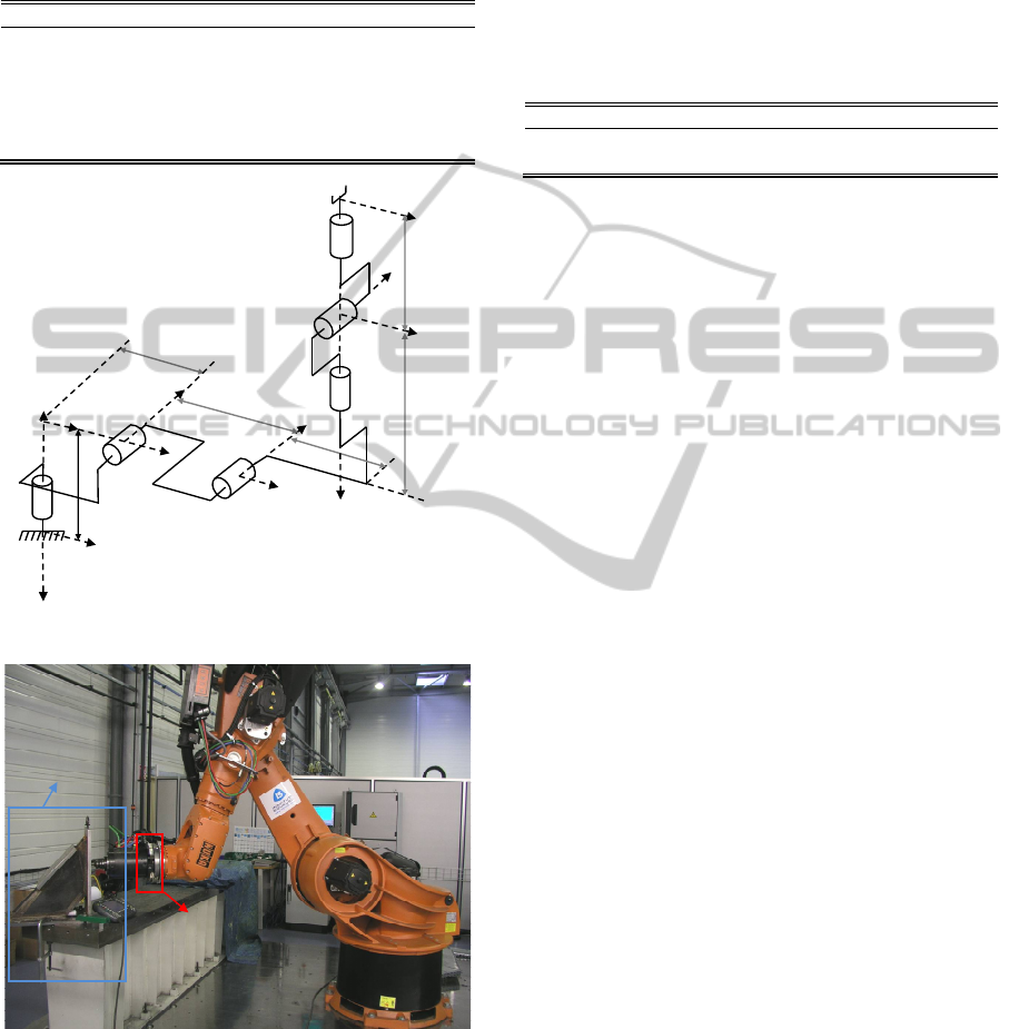
4.1 Modeling of the Kuka KR500
The Kuka KR500 robot (see figure 2) has a serial
structure with n=6 rotational joints. Its kinematics is
defined using the Modified Denavit and Hartenberg
(MDH) notation (Khalil and Kleinfinger, 1986). In
this notation, the link j fixed frame is defined such
that the z
j
axis is taken along joint j axis and the x
j
axis is along the common normal between z
j
and z
j+1
(see figure 1).
j
and d
j
parameterize the angle and
distance between z
j-1
and z
j
along x
j-1
, respectively,
whereas
j
and r
j
parameterize the angle and distance
between x
j-1
and x
j
along z
j
, respectively. All MDH
positions are equal to the motor position q
mj
given by
the KRL controller of the Kuka KR500 except for
axis 3 and 6. The geometric parameters are given in
table 1 and allow to compute the (6x6) jacobian
matrix (3). All variables are given in SI unit in joint
link side. The robot is characterized by a kinematic
JointStiffnessIdentificationofaHeavyKukaRobotwithaLow-costClampedEnd-effectorProcedure
587
coupling effect between the joint 4,5 and 6 but his
impact is negligible because the coupling
coefficients are very low (Jubien and Gautier, 2013).
Table 1: MDH parameters of the KR500 robot.
j
j
d
j
j
r
j
1
0 q
m1
rl
1
(= -1.045 m)
2
d
2
(= 0.500 m) q
m2
0
3
d
3
(= 1.300 m)
q
m3
0
4
d
4
(= -0.055 m) q
m4
rl
4
(= -1.025 m)
5
0 q
m5
0
6
0
q
m6
rl
6
(= -0.290 m)
6
x
5
z
6
rl
45
,
x
x
4
rl
46
,zz
4
d
3
z
3
x
3
d
2
z
2
d
2
x
1
rl
1
x
0
z
0
x
Figure 1: Link frame of the KR500 robot.
ATI force sensor
L
ockin
g
s
y
stem
Figure 2: Picture of robot on configuration 2.
4.2 Configuration of the Robot with
Fixed End-effector
The ATI force sensor used does not allow the
simultaneous measurement of the three components
of f
e
and of three components of m
e
. In our case,
only the component f
z
is measured. Therefore, it is
necessary to chose some configurations of robot
where the other components of the wrench are fixed
at zeros values.
To do this, two configurations of the robots are
studied to identify the joint stiffness of axis 1 and 2.
There are given in table 2.
Table 2: Configurations of the KR500 robot.
Conf. nb q
1
q
2
q
3
q
4
q
5
q
6
1 1.62 -0.89 1.84 1.62
0.46
2 1.48 -0.87 1.37
-1.05 0
The first configuration allows identifying the
joint stiffness of axis 1. The second (see figure 2)
configuration allows identifying the joint stiffness of
axis 2. Thus, it is possible to identify joint stiffness
parameters without the measurement of all
components of the wrench (except for axis 6).
4.3 Acquisition, Trajectories and
Filtering
The sampling acquisition frequency of force sensor
is 83.3(Hz) and the sampling acquisition frequency
of motor currents and motor positions is 500(Hz).
All the measurements are synchronized off-line. The
motor currents and motor positions are given by
'Scope' function of Kuka KRC controller.
For each configuration, the end-effector of the
robot is bought into contact with the rigid
environment with position control. After that, the
robot is controlled with force control and different
levels of force on z
6
are applied on the end-effector
to have a significant number of points. The end-
effector is blocked only on the same direction z6,
accordingly the component f
z
can be only negative.
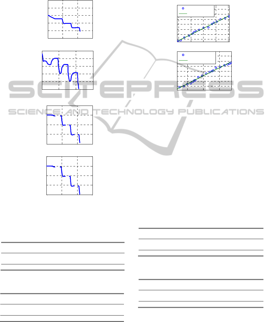
The motor positions, currents, external torques and
measurement of f
z
for the configurations 1 are given
in figure 3. f
z
cannot be measured all the time due to
restriction on acquisition system so only the
available measurements are showed for f
z
and the
external torques.
For the identifications, the cut-off frequency of
the Butterworth filter is fixed to 10Hz and the cut-
off frequency of decimate filter is fixed to 5Hz.
4.4 Identification of Joint Stiffness with
Motor Currents
The identification of the joint stiffness of axis 1 and
2 are performed with motor currents and motor
positions. The IDIM (8) is used and the motor
ICINCO2014-11thInternationalConferenceonInformaticsinControl,AutomationandRobotics
588
torques are computed with (9). The parameters of
each axis are identified separately. The identified
values of joint stiffness and offset are given in table
3 and 4.
0 5 10 15
1.6225
1.623
1.6235
1.624
1.6245
1.625
Time (s)
q
m1
(rad)
0 5 10 15
-8
-6
-4
-2
0
2
Time (s)
I
1
(A)
0 5 10 15
-6000
-4000
-2000
0
2000
Time (s)
o1
(Nm)
0 5 10 15
-3000
-2000
-1000
0
1000
Time (s)
f
z
(N)
Figure 3: Motor position, motor current and joint torque
for axis 1 and force (configuration 1).
Table 3: Identified stiffness value with motor torques for
axis 1.
Par.
ˆ
χ
ˆ
%
r
k
1
6.09 10
6
2.1
Offkm
1
-9.90 10
6
2.1
|Wχ-Y|/|Y| 2.82%
Table 4: Identified stiffness value with motor torques for
axis 2.
Par.
ˆ
χ
ˆ
%
r
k
2
8.00 10
6
2.0
Offkm
2
6.93 10
6
2.1
|Wχ-Y|/|Y| 2.67%
The stiffness parameters are well identified with
a low relative standard deviation. The motor torque
(circle) relative to motor position for axis 1 and 2 is
showed in figure 4. A green line (
ˆ
ˆ
j
mj j
kq Offkm ) is
drawn for comparison.
1.586 1.5862 1.5864 1.5866 1.5868
-6000
-5000
-4000
-3000
-2000
-1000
0
q
1
(rad)
m1
(Nm)
k
1
q
1
+ Offkm
1
(Nm)
-0.8462 -0.846 -0.8458
3000
4000
5000
6000
7000
8000
9000
q
2
(rad)
m2
(Nm)
k
2
q
2
+ Offkm
2
(Nm)
Figure 4: Variation of motor torque relative to variation of
motor position for axis 1 and 2.
4.5 Identification of Joint Stiffness with
Wrench
The identification of the joint stiffness of axis 1 and
2 is performed with wrench and motor positions.
The IDIM (11) is used and the joint torques are
computed with (12). The jacobian matrix is
computed from motor positions and with DHM
parameters given in table 1. The parameters of each
axis are identified separately. The identified values
of joint stiffness and offset are given in table 5 and
6.
Table 5: Identified stiffness value with external torques for
axis 1.
Par.
ˆ
χ
ˆ
%
r
k
1
6.93 10
6
0.77
Offkl
1
-1.12 10
7
0.78
|Wχ-Y|/|Y| 1.44%
Table 6: Identified stiffness value with external torques for
axis 2.
Par.
ˆ
χ
ˆ
%
r
k
2
7.81 10
6
0.98
Offkl
2
6.76 10
6
0.97
|Wχ-Y|/|Y| 2.13%
As above, the stiffness parameters are well
identified with a low relative standard deviation
JointStiffnessIdentificationofaHeavyKukaRobotwithaLow-costClampedEnd-effectorProcedure
589
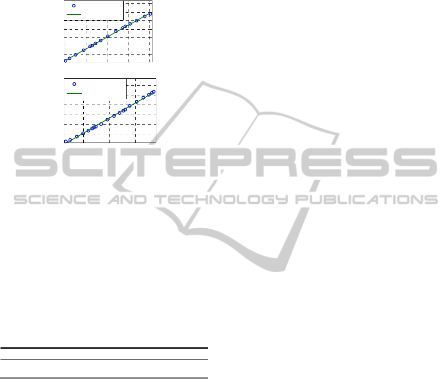
(<1%). The external torque (circle) relative to motor
position for axis 1 and 2 is showed in figure 5. A
green line (
ˆ
ˆ
j
mj j
k q Offkl ) is drawn for comparison.
1.586 1.5862 1.5864 1.5866 1.5868
-5000
-4000
-3000
-2000
-1000
0
1000
q
1
(rad)
o1
(Nm)
k
1
q
1
+ Offkl
1
(Nm)
-0.8462 -0.846 -0.8458
1000
2000
3000
4000
5000
6000
q
2
(rad)
o2
(Nm)
k
2
q
2
+ Offkl
2
(Nm)
Figure 5: Variation of external torque relative to variation
of motor position for axis 1 and 2.
4.6 Comparison and Discussion
The relative differences between the identified
stiffness values with motor currents and wrench are
given in table 7. The two methods work well to
identify the joint stiffness parameters and give
similar results. The differences may come from the
precision of the a priori joint drive gain in (9), the
precision of the ATI sensor, the precision of the
MDH parameters and the approximation J(q)≈J(q
m0
).
Table 7: Relative errors between identified stiffness
parameters with motor and external torques.
Par.
%e
k
1
12.1%
k
2
2.43%
The major advantage of our methods is that they
avoid the measurement of joint positions and/or the
attitude measurement of end-effector and the use of
additional payload. The position measurement of
end-effector requires very expensive external
measurement systems. Here, it is possible to identify
the joint stiffness with and without the measurement
of the wrench.
The measurement of the wrench needs a force
sensor. Some robots are already equipped with this
sensor to perform force control otherwise it must be
installed. But our approach allows avoiding the use
of wrench using only motor current if using of force
sensor is too difficult.
We recall that in practice, the identified stiffness
values with our model are the addition of the actual
joint stiffnesses and some of the link stiffnesses.
To achieve this ,it is needed to clamp the end-
effector to the environment which is easy if you use
a beam, the soil or a vise on a production line or in a
laboratory.
Unlike the method proposed in (Dumas et al.,
2011), our method avoids optimizing the robot
configuration to minimize its complementary
stiffness matrix since the end-effector is clamped
(i.e. it does not move). If only the motor torques are
used, the computation of jacobian matrix and its
condition number are no longer necessary.
The experimental validation on the two first axis
of an industrial robot shows the effectiveness of our
method.
5 CONCLUSION
This paper shows that it is possible to accurately
identify static joint stiffnesses of industrial robots
with a low-cost and easy to use procedure based on
clamping the end-effector to the environment. The
strong result is that the identification using only
internal measurements of motor positions and
torques gives similar results to those obtained with
force sensor measurements of the interaction
wrench. The method can be carried out on industrial
robots without the need of any external sensor like
expensive laser tracker or force sensor. It is a first
validation of our methodologies on a simple case.
Future works concern the identifications of all joint
stiffness of the robot and a comparison with other
joint stiffness identification methods .
ACKNOWLEDGEMENTS
This work was supported by the French ANR
COROUSSO ANR-2010-SEGI-003-02-
COROUSSO.
REFERENCES
Alici, G., Shirinzadeh, B., 2005. Enhanced Stiffness
Modeling, Identification and Characterization for
Robot Manipulators. IEEE Transactions on Robotics
21, 554–564.
Dumas, C., Caro, S., Garnier, S., Furet, B., 2011. Joint
Stiffness Identification of Six-revolute Industrial
ICINCO2014-11thInternationalConferenceonInformaticsinControl,AutomationandRobotics
590

Serial Robots. Jour of Robotics and Computer
Integrated Manufacturing.
Gautier, M., 1997. Dynamic identification of robots with
power model. IEEE International Conference on
Robotics and Automation, IEEE, pp. 1922–1927.
Gautier, M., Jubien, A., Janot, A., Robet, P.-P., 2013.
Dynamic Identification of Flexible Joint Manipulators
with an Efficient Closed Loop Output Error Method
Based on Motor Torque Output Data. IEEE
International Conference on Robotics ans Automation.
Gautier, M., Khalil, W., 1990. Direct calculation of
minimum set of inertial parameters of serial robots.
IEEE Transactions on Robotics and Automation 368–
373.
Hollerbach, J., Khalil, W., Gautier, M., 2008. Model
Identification, in: Springer Handbook of Robotics.
Springer.
Janot, A., Gautier, M., Jubien, A., Vandanjon, P.O., 2011.
Experimental joint stiffness identification depending
on measurements availability. IEEE Conference on
Decision and Control and European Control
Conference, pp. 5112–5117. doi:10.1109/CDC.2011.
6160402
Janot, A., Vandanjon, P. O., Gautier, M., 2014. A Generic
Instrumental Variable Approach for Industrial Robot
Identification. IEEE Transactions on Control Systems
Technology 22, 132–145.
Jubien, A., Gautier, M., 2013. Global identification of
spring balancer, dynamic parameters and drive gains
of heavy industrial robots. IEEE/RJS International
Conference on Intelligent Robots and Systems, pp.
1355–1360.
Khalil, W., Dombre, E., 2002. Modeling, Identification
and Control of Robots, 3rd edition. ed. Taylor and
Francis Group, New York.
Khalil, W., Kleinfinger, J., 1986. A new geometric
notation for open and closed-loop robots. IEEE
International Conference on Robotics and
Automation, pp. 1174–1179.
Östring, M., 2003. Closed-loop identification of an
industrial robot containing flexibilities. Control
Engineering Practice 291–300.
Pfeiffer, F., Holzl, J., 1995. Parameter identification for
industrial robots. IEEE International Conference on
Robotics and Automation, IEEE, pp. 1468–1476.
doi:10.1109/ROBOT.1995.525483
Pham, M. T., Gautier, M., Poignet, P., 2001. Identification
of joint stiffness with bandpass filtering. IEEE
International Conference on Robotics and
Automation, pp. 2867–2872. doi:10.1109/ROBOT.
2001.933056.
JointStiffnessIdentificationofaHeavyKukaRobotwithaLow-costClampedEnd-effectorProcedure
591
