Extending the Software Tool TimeNET

by Power Consumption Estimation of UML MARTE Models

Dmitriy Shorin and Armin Zimmermann

System & Software Engineering, Technische Universit

at Ilmenau, P.O. Box 100 565, D-98684 Ilmenau, Germany

Keywords:

UML, MARTE, Petri Net, Power Consumption, System Design, Modeling Tool TimeNET.

Abstract:

This paper presents an extension of the software tool TimeNET, which supports modeling and analysis of

stochastic Petri nets. The new extension implements a previously proposed method for power consumption

modeling and evaluation based on extended UML models. Two new net classes have been developed to

support the necessary operational and application models and edit them in the graphical user interface. Several

stereotypes of the UML Proﬁle for Modeling and Analysis of Real-Time and Embedded Systems (MARTE)

have been added to extend the information about power consumption of system and application states. The

two UML models are then automatically transformed into a stochastic Petri net. Power consumption of the

system can be predicted by standard Petri net analysis modules of TimeNET. An example of an industrial

control system is provided.

1 INTRODUCTION

Energy consumption is an increasingly important

non-functional property of embedded systems and in

automation in general. Design decisions have to be

based on a trade-off between energy use and other re-

quirements. It is thus important to evaluate the ef-

fect of architectural and other design decisions in all

phases of the development process based on a good

prediction of the energy consumption of an embed-

ded system. In this work, we concentrate on early

design steps, in which major architectural decisions

are made, which may have a signiﬁcant impact on

the overall system’s energy consumption. Modeling

methods should be developed for discrete automation

systems in such a way that the energy consumption,

beside other parameters, can be modeled, estimated,

and ﬁnally reduced.

The Uniﬁed Modeling Language (UML) (Object

Management Group (OMG), 2012) is an industry

standard for describing software systems. However,

it is not intended to describe non-functional system

properties equally well, as there are no constructs

for quantitative properties. Domain proﬁles of the

UML have been developed for this task, namely,

the MARTE proﬁle (Modeling and Analysis of Real-

Time and Embedded Systems (Object Management

Group (OMG), 2011)) as a successor of the UML SPT

proﬁle (Object Management Group (OMG), 2005).

UML models adopting the MARTE proﬁle con-

tain the necessary information for energy consump-

tion estimation. However, they are not usable di-

rectly, as UML models are not semantically well-

deﬁned for a speciﬁcation of the resulting stochas-

tic process. For this work, we proposed UML mod-

els to be transformed into a model for which anal-

ysis algorithms exist and, namely, into extended de-

terministic and stochastic Petri nets (eDSPN) (Ger-

man, 2000), such that the behavior and the proper-

ties are preserved. This was motivated by an earlier

work by a former colleague, in which single extended

UML state chart models describing reliability aspects

of a system were transformed into uncolored SPNs for

their analysis (Trowitzsch and Zimmermann, 2005;

Trowitzsch, 2007).

The proposed method has been described in de-

tail in (Shorin et al., 2012), covering how the energy

consumption of a microcontroller can be estimated

by dividing the system into hardware and software

parts. The hardware part remains the same for all

applications, and is thus described in an operational

model and speciﬁes all possible modes of the system,

the possible state changes, and their associated power

consumption (as well as transition times, if applica-

ble).

On the other hand, the effect of the controlling

software is captured in one or more application mod-

els. It describes which steps are taken and what time

Shorin D. and Zimmermann A..

Extending the Software Tool TimeNET by Power Consumption Estimation of UML MARTE Models.

DOI: 10.5220/0005096700830091

In Proceedings of the 4th International Conference on Simulation and Modeling Methodologies, Technologies and Applications (SIMULTECH-2014),

pages 83-91

ISBN: 978-989-758-038-3

 2014 SCITEPRESS (Science and Technology Publications, Lda.)

is spent in which mode, and may have stochastic be-

havior (interrupts, for instance). Thus, it contains

information about the operational states used in the

speciﬁed system and their duration. The model dis-

tinction follows the principle of separation of con-

cerns in (software) engineering of complex systems.

This type of distinction can be found in other ﬁelds

as well, for instance in manufacturing systems, where

a similar relation exists between structure (machines,

transport routes) and work plans (Zimmermann and

Hommel, 1999).

The two models together contain all the necessary

information for predicting the power consumption. In

this paper, we present an extension of the software

tool TimeNET (Zimmermann, 2012) that makes pos-

sible an automatic combined transformation into an

SPN. The resulting model can then be used to esti-

mate the power consumption of the system with sta-

tionary analysis.

A related approach similar to the one of (Trow-

itzsch and Zimmermann, 2005; Trowitzsch, 2007) is

taken in (Callou et al., 2008), in which enriched UML

models are translated into stochastic Petri nets. The

main difference to our work is the distinction between

the two aspect models and their integration during

transformation. Another approach with similar goals

is presented in (Andrade et al., 2009), where a UML

model is translated into a colored Petri net (CPN)

description as supported by the CPN tools (Jensen

et al., 2007). However, the resulting model tends to

be rather complex and the CPN interpretation does

not support a natural notion of (stochastic) time sim-

ilar to the widely accepted model class of stochastic

Petri nets.

The paper is structured as follows. Section 2

brieﬂy recalls the implemented method. Section 3 de-

scribes the tool environment TimeNET and the imple-

mented extension. An example is presented in Sec. 4,

before some ﬁnal conclusions and acknowledgments

are given.

2 METHOD DESCRIPTION

We consider each embedded system to be consist-

ing of hardware and software parts. The hard-

ware part of the system is reﬂected in the opera-

tional model. In this model, all possible states and

transitions of the system itself (without application-

dependent speciﬁcs) must be described. One embed-

ded system can be described by means of only one

operational model, as the hardware part of an embed-

ded system are more stable than the software. In case

of a change in the components of the embedded sys-

tem under consideration, a new or adapted operational

model is needed.

The software part of the system is described in the

application model. This model contains information

about the states of each of the speciﬁed programs run-

ning on the system, their waiting times and duration.

Any modiﬁcation of the software part of the system

must be reﬂected in the application model, yet the op-

erational model remains the same. Thus, any embed-

ded system can be represented by means of a single

operational model and an set of application models.

For building both models, we use the means of one of

the behavioral UML diagrams – State Machine Dia-

gram – extended with the stereotypes of the MARTE

proﬁle.

2.1 Operational Model

This model contains all the necessary information

for analyzing the (hardware) system under considera-

tion. All possible states and transitions of the system

should be described, and all state names have to be

unique to avoid ambiguities as the later application

model identiﬁers correspond to them.

The states are described by means of the

<<ResourceUsage>> stereotype of the MARTE

proﬁle. This package was specially created for con-

sidering the resource consumption in the system. Two

attributes are taken into account: execTime and pow-

erPeak. The ﬁrst one reﬂects the duration of staying

in each state (in seconds), while the second represents

the power required for the state (in Watt).

All the simple states must have an attribute pow-

erPeak that speciﬁes the power consumption of the

simple states. The attribute execTime should be ap-

plied if the (default) execution time for some simple

states is known and remains the same regardless of

the application executed.

2.2 Application Model

At the second stage of the proposed method, an ap-

plication model has to be created. It contains infor-

mation about the states used in the speciﬁed program

and their duration. The order of transitions between

the modes must comply with the order speciﬁed in the

operational model. However, the states for which both

the power consumption and the execution time are

given in the operational model may be skipped in the

application model. For the correspondence detection

between these two models, the modes implemented in

the application model must be named identical to the

states of the operational model. It is required to mark

the initial state of the system.

SIMULTECH2014-4thInternationalConferenceonSimulationandModelingMethodologies,Technologiesand

Applications

The attribute execTime has to be applied by all

simple states if it is not stated in the operational

model. It speciﬁes the execution time of the simple

states. If the execution time is given in both opera-

tional and application models, the value from the ap-

plication model will be taken for the analysis. This

decision lets the user overwrite the default execution

time if necessary.

The attribute prob has to be given for all the states

which immediately follow the choice pseudostate. It

speciﬁes the execution probabilities for these follow-

ing states.

As it is impossible to set attributes by pseu-

dostates, transitions going out of the choice pseu-

dostate must lead only to the simple states. This is

a known UML problem. If this rule is not followed,

the system model will be incompletely speciﬁed.

2.3 Transformation Rules

For analyzing the energy consumption of the system,

we combine application and operational models and

convert them into a Petri net. For this operation, we

take the application model as the basic one. The oper-

ational model delivers the missing information, such

as power consumption, missing states, and their dura-

tion.

For each simple state of the application model,

there must be a certain simple state in the operational

model. Simple states of the operational model can be

either linked to one, several, or no simple states in the

application model.

States and their outgoing transitions are trans-

formed simultaneously, because UML transitions af-

ter different state types are transformed either into ex-

ponential or immediate transitions.

The rules used to transform UML models into

a Petri net are described in detail in (Shorin et al.,

2012).

Each UML simple state of the application model

with its outgoing transition is transformed into a Petri

net place and a transition if such transition between

two states exists in the operational model. If this is

not the case and such transition does not exist in the

operational model, the path must be found through

the other states in the operational model, for which all

the necessary information (execution time and power

consumption) is given. If more than one way exists,

the software tool warns the user and chooses the one

in which the system consumes less power. The well-

known Dijkstra algorithm (Dijkstra, 1959) was imple-

mented in the software tool for this task.

Each execution time value of the simple states is

transformed into the attribute delay of the appropriate

exponential transition of the Petri net.

Each UML simple state of the application model

has its power consumption. The relevant value is

taken from the linked simple state of the operational

model. The formula for power consumption estima-

tion represents a sum of the probabilities of the state

activation multiplied with its power consumption val-

ues. The calculation result is then added as a perfor-

mance measure object of the Petri net in TimeNET.

measure =

∞

∑

i=1

P(#state

> 0) · powerPeak(#state

)

(1)

Each UML choice pseudostate of the application

model is transformed into a Petri net place which is

followed only by immediate transitions that model the

probabilistic choice.

Every UML join pseudostate of the application

model is transformed into a Petri net place which is

followed by an immediate transition. Each value prob

of the simple states, which immediately follow UML

choice pseudostates, is transformed into the attribute

weight of the appropriate immediate transition of the

resulting Petri net.

Each UML initial state is transformed into a Petri

net place which is followed by an immediate tran-

sition. The attribute initialMarking of the Petri net

place is then set to 1.

After ﬁnishing the UML model transformation,

the power consumption can be automatically calcu-

lated either by a numerical analysis or simulation

both in transient and steady-state by algorithms of

TimeNET.

3 TOOL IMPLEMENTATION AS

A TIMENET EXTENSION

This section presents TimeNET – a software tool

for modeling and evaluation of stochastic Petri nets.

Subsection 3.1 gives some general information about

the software tool. An earlier work added stochas-

tic UML state charts (Trowitzsch and Zimmermann,

2005; Trowitzsch, 2007) to the tool (Trowitzsch et al.,

2007). This existing extension was primarily aimed at

reliability modeling and evaluation. The current paper

presents the further extension of the tool by energy

use description and evaluation. The main difference

to (Trowitzsch et al., 2007) is the distinction between

operational and application models as described in

Sec. 2. Subsection 3.2 describes in detail the integra-

tion of the new extension into TimeNET, especially

corresponding to the two new necessary net classes.

The tool functionality is presented in Subsec. 3.3.

ExtendingtheSoftwareToolTimeNETbyPowerConsumptionEstimationofUMLMARTEModels

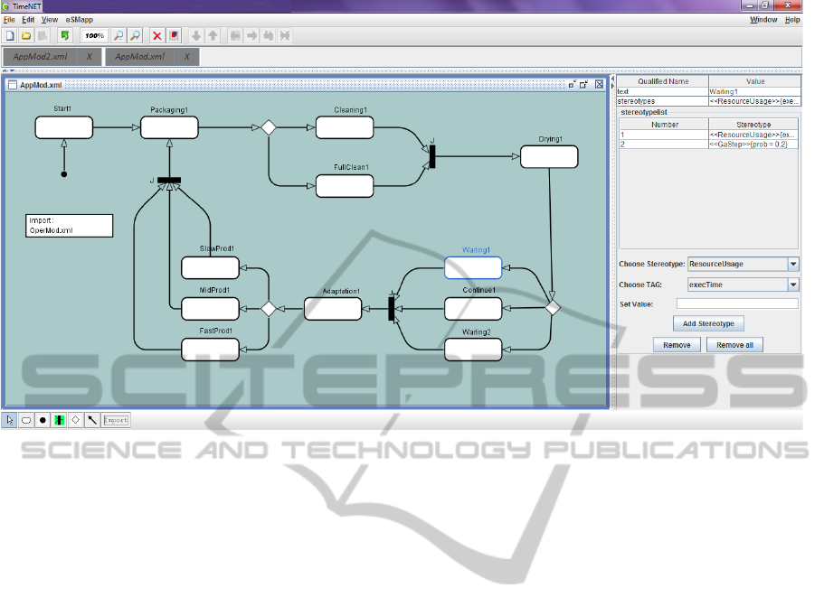
Figure 1: Application model built in TimeNET.

3.1 Tool Description

TimeNET (Zimmermann, 2012; German et al., 1995)

is a software tool supporting modeling and perfor-

mance evaluation of stochastic Petri nets, especially

for models with non-exponentially distributed ﬁring

delays (German, 2000). TimeNET analyses extended

stochastic Petri nets and colored stochastic Petri nets.

The software also lets the user create UML state

charts, which will be then transformed into stochas-

tic Petri nets for the further analysis.

The software tool has been originally built at the

Technische Universit

at Berlin and is being developed

by the System and Software Engineering group of

the Technische Universit

at Ilmenau since 2008. The

functionality of the software is being continuously ad-

vanced, so that it covers more and more aspects of

Petri net analysis and related models. The modular

tool architecture lets computer engineers extend the

program code easily and thus, enlarge the possibili-

ties of the software. The current version of the soft-

ware 4.2 appeared in May 2014 at the time of the pa-

per writing.

The interactions between components of

TimeNET are well described in (Zimmermann,

2012). The central connecting module is the graph-

ical user interface (GUI). It is programmed in Java

for portability and uses data and model schemata

speciﬁed in XML (eXtensible Markup Language).

The GUI calls different simulation and analysis

algorithms as requested by the user. These compo-

nents are written in C and C++, often including code

generated at run time for efﬁciency reasons.

After starting the simulation process, the GUI cre-

ates a master process. It gathers all the given parame-

ters of the user models and compiles all the necessary

information from the GUI. It then starts slave pro-

cesses which execute the actual simulation. The in-

teraction between GUI and analysis algorithms is re-

alized with data ﬁles, while sockets are used between

analysis processes. The master process controls in-

teractions between slave processes and, ﬁnally, reads

the results. These are sent to the GUI where they are

presented to the user.

TimeNET can be used in both Linux- and

Windows-based operating systems. The GUI (PENG,

platform-independent editor for net graphs (Jakop,

2003)) is generic and lets the user easily implement

any graph-like modeling formalism. Thus, TimeNET

is not restricted to stochastic Petri nets, but can be

extended for using other graphs such as UML state

charts or automata.

The software can be extended by new net classes

which use speciﬁc algorithms. While creating a new

model in TimeNET, the user chooses the applicable

net class and the GUI is being extended by the re-

spective algorithms.

The main window of TimeNET (see Fig. 1) in-

cludes a standard menu panel which lets the user work

with ﬁles, edit models, change the model’s view and

choose one of the algorithms speciﬁc for the current

net class. For example, for building the model in

SIMULTECH2014-4thInternationalConferenceonSimulationandModelingMethodologies,Technologiesand

Applications

Table 1: Stereotypes and attributes used in the models.

Stereotype Attribute Operational model Application model

<<ResourceUsage>> powerPeak mandatory not applicable

execTime optional mandatory

<<GaStep>> prob optional mandatory

Fig. 1, we used the net class eSMapp, one of the two

net classes described further in this paper. The de-

tailed information is presented in Subsec. 3.3.

The toolbar below the menu panel contains but-

tons for the most frequently used commands. The

next toolbar from the top lets the user switch between

models opened in the software tool. The main part of

the window is occupied by the graphical workspace

for building models. The model elements which can

be used in the given net class are shown below the

main window in the icon bar at the left. The panel on

the right-hand side serves for changing model element

properties and adding attributes.

The user’s interaction with the GUI does not dif-

fer from common standards. The user chooses an

element in the bar at the bottom of the screen and

clicks on the workspace to place it. In the mode se-

lect, which is depicted by a white arrow, the user can

move elements in the workspace, edit them and state

their parameters in the list on the right-hand side.

3.2 Integration of Energy-Aware State

Machines in TimeNET

For estimating power consumption, two new net

classes were implemented in TimeNET. Both deal

with energy-aware UML state charts (eSM). The op-

erational model is being created within the net class

eSMoper, the other net class eSMapp serves for cre-

ating application models such as described in Sec. 2

and previous papers (Shorin et al., 2012; Shorin and

Zimmermann, 2013). They have similar structure, but

support the differences between two types of models

described in Sec. 2. The XML schemata implemented

for these net classes are based on the schema for the

net class sSM, which was created for modeling UML

stochastic state machines (Trowitzsch et al., 2007).

A necessary subset of UML elements described in

Sec. 2 was implemented in the current prototype and

can thus be used in the given net classes.

Figure 2 depicts the integration of the net classes

eSMoper and eSMapp into TimeNET. Using the

TimeNET GUI, the user can build operational and ap-

plication models by means of these two net classes.

The models will be saved in two XML ﬁles. Any ap-

plication model has to be conceptually linked to an

operational model — this relation is provided by the

user in the application model (details in Subsec. 3.3).

Graphical User Interface

eSMoper

net class

XML Schema

eSMoper

model

XML file

eSMapp

net class

XML Schema

eSMapp

model

XML file

eDSPN

model

XML file

eDSPN

net class

XML Schema

Transformation

Stationary

analysis

Figure 2: Integration of eSMoper and eSMapp net classes.

Each net class has its speciﬁc functions, which are

represented in the menu bar. Thus, the user can

start the transformation into an eDSPN model only

while using the net class eSMapp. The command

starts the conversion based on the rules given in Sub-

sec. 2.3. During this procedure, the information from

two models is being merged and a ﬁnal SPN is thus

being created (Shorin et al., 2012). The resulting Petri

net belongs to the net class eDSPN, the fundamental

class of TimeNET, for which analysis and simulation

functions are available. The stationary analysis of the

Petri net results in the estimated power consumption

of the analyzable system.

The net classes eSMoper and eSMapp provide

the user only with the UML state chart elements de-

picted further in Fig. 3. Thus, they support model-

ing of simple states, initial, join, and choice pseu-

dostates, as well as transitions. Simple states can be

extended by some stereotypes of the MARTE pro-

ﬁle. The stereotype <<ResourceUsage>> is being

used here for specifying power consumption (attribute

powerPeak) and execution time (attribute execTime)

of the simple states. The tag prob of the other stereo-

type <<GaStep>> serves for setting the probabili-

ties of the states which immediately follow the choice

pseudostate. Table 1 indicates the stereotypes and

tags supported by the net classes and shows if they

are mandatory in operational and application mod-

els. Furthermore, state machines built in these two

classes must fulﬁll the conditions given in the method

description (Sec. 2).

3.3 Tool Functionality

Figure 1 shows the GUI while creating an applica-

tion model. The menu panel includes section eSMapp

which contains functions speciﬁc for the net class. Its

function eSMapp to eDSPN converts two models into

ExtendingtheSoftwareToolTimeNETbyPowerConsumptionEstimationofUMLMARTEModels

SPN for further analysis. The icon bar on the bot-

tom of the screen includes following modeling ele-

ments: mode select, simple state, initial, join, and

choice pseudostates, state transition, and element Im-

port. The last one can be used to set the operational

model linked to the current application model.

The TimeNET window while working in the net

class eSMoper looks similar with two exceptions: The

section eSMoper of the menu panel does not let the

user create an SPN out of the operational model, and

the icon bar at the bottom of the screen does not in-

clude the element Import. The reason for this is that

one operational model can be linked to numerous ap-

plication models.

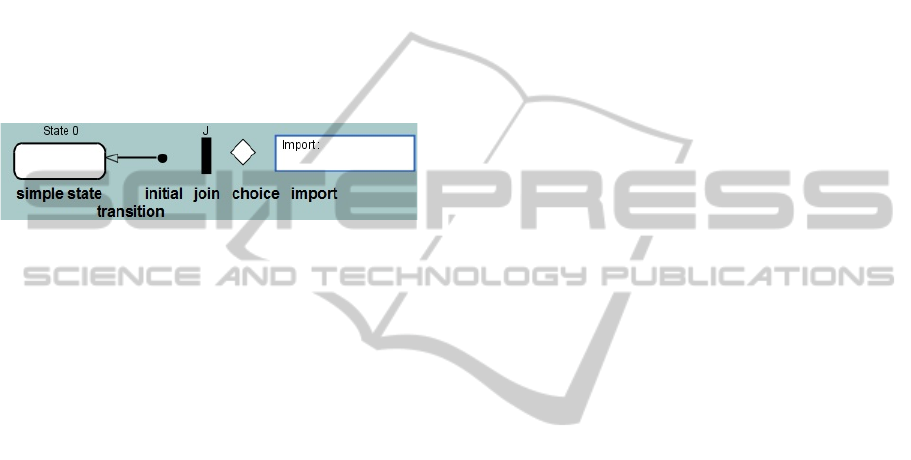
Figure 3: Elements for creating an application model.

Elements which can be used for creating an appli-

cation model are shown in Fig. 3. A simple state is

represented by an empty rectangle with rounded cor-

ners. The initial pseudostate is depicted as a small

solid black circle. The join pseudostate is shown as

a small solid black rectangle with a letter J above it,

while the choice pseudostate is depicted as an empty

rhombus. Transitions are displayed as an arrow di-

rected from the outgoing state to the incoming state.

The Import speciﬁcation is represented by an empty

rectangle with standard sharp corners. Inside the ﬁg-

ure, there is a word Import with a semicolon and

the name of the ﬁle containing the operational model

linked to the current application model.

By selecting a simple state in the selection mode,

the user can add attributes and change its name in

the panel at the right side of the screen (see Fig. 1).

Initially, each simple state gets a name which con-

sists of the word ”state” and an ordinal number be-

ginning from zero automatically. The user has the

opportunity to change the name in the property text.

The property stereotype is being used for adding at-

tributes to the element. This ﬁeld can be ﬁlled up

automatically by using the ﬁelds below. The stereo-

typelist demonstrates all the attributes added to the

chosen state. In the ﬁeld Choose stereotype, the

user can choose between <<ResourceUsage>> and

<<GaStep>> stereotypes. Depending on the choice

in this ﬁeld, the ﬁeld Choose TAG offers to state

either execution time in the attribute execTime (in

the case of the <<ResourceUsage>> stereotype) or

the state probability in the attribute prob (stereotype

<<GaStep>>). By creating an operational model,

the attribute powerPeak of the <<ResourceUsage>>

stereotype is also available for stating the power con-

sumption of the simple state. This attribute is not

available in the application model as it is stipulated

by the method described in Sec. 2. Table 1 gives an

overview of the attributes which can or must be used

in both models. In the text ﬁeld Set Value, the user

states a value of the chosen attribute. By clicking

the button Add Stereotype, the chosen attribute will

be added to the stereotype list above. The further but-

tons Remove and Remove all let the user delete either

a single chosen attribute or all of them, respectively.

The element Import has an additional property

ﬁeld ﬁlename, which is used to set the name of the

XML ﬁle containing the corresponding operational

model.

After creating both operational and application

model, the user can start the transformation to a Petri

net via the menu item eSMapp → eSMapp to eDSPN.

TimeNET will ask for the name of the resulting XML

ﬁle to save the results. After the transformation,

the created ﬁle containing a new eDSPN should be

opened and the stationary analysis (menu Evaluation)

started. The results will be displayed in the ﬁeld mea-

sure in the TimeNET workspace. The value gives an

estimation of the system power consumption.

4 EXAMPLE

In this section, we show how the possibilities of the

presented TimeNET extension are used in practice.

In comparison to the example given in (Shorin et al.,

2012), we explicitly take not an embedded, but an

industrial control system to show the breadth of the

method and software application. In this example, we

consider component production by a workbench with

a main and two reserve motors. Its structure is de-

picted in Fig. 4.

The workbench gets its ﬁrst order and is being

started (represented by the state Start). The process

goes through the ﬁctitious state Continue (see details

below) and the order is adapted. Furthermore, there

are three possibilities of producing components de-

pending on performance requirements. The ﬁrst one

is called Slow production — it takes 5 minutes to cre-

ate one unit. By choosing the second mode, one mo-

tor more is started and thus, the production speed re-

duces to 3 minutes. The third possibility is to start

two reserve motors and to produce the component in

only one minute. The fastest way could be the most

preferable one, but the difference between these three

modes is also in the power consumption. We assume

that the longer it takes the workbench to produce a

SIMULTECH2014-4thInternationalConferenceonSimulationandModelingMethodologies,Technologiesand

Applications

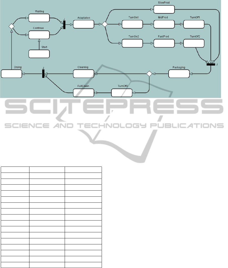
Figure 4: Operational model of the workbench.

unit, the less overall power it needs for this opera-

tion. The energy needed for the workbench to func-

tion in the ﬁrst mode is 2.5 watt-seconds, in the sec-

ond one 3 W·s and in the third – 5 W·s. Thus, the

example could be used to show a design trade-off be-

tween power consumption and other conﬂicting non-

functional properties of a system. An overview of the

attributes related to the states is given in Table 2.

Table 2: Attributes stated in the operational model.

State name powerPeak, W execTime, min.

Start 5 2

Waiting 0.1

Continue 0 0.00001

Adaptation 0.2 0.1

TurnOn1 2 0.2

TurnOn2 4 0.2

SlowProd 0.5 5

MidProd 1 3

FastProd 5 1

TurnOff1 0.1 0.1

TurnOff2 0.2 0.1

TurnOff3 0.1 0.4

Packaging 0.3 0.2

Cleaning 0.3 0.1

FullClean 1 0.5

Drying 0.4 0.1

If one or two reserve motors are used in the pro-

duction process, it takes extra time and power to turn

them on and off (states TurnOn1, TurnOn2, TurnOff1,

TurnOff2). When the component is produced, it

will be packed (Packaging). After each procedure,

the workbench must be cleaned. Cleaning has two

modes: either a normal quick Cleaning or a Full

Cleaning which takes more time and demands the

main motor to be also stopped (TurnOff3). After that,

it takes a little time to dry the workbench (Drying).

If necessary, the main motor is being started during

this process. Thus, the workbench ﬁnishes its work

on the unit and goes either in the standby mode (Wait-

ing) or continues its work without a pause. The value

0.00001 given in the Continue state is caused by the

requirement for the exponential transitions of Petri

net: the delay value which here represents the exe-

cution time may not be equal to zero. Otherwise, the

Petri net will not be properly analyzable. However,

this substitution does not inﬂuence the end result. The

only function of the state Continue itself is to be a reg-

ular (non-pseudo) state after the choice pseudostate.

This restriction of UML was described in Subsec. 2.2.

Figure 4 depicts the operational model built on the

basis of the system description above. After that, the

user can create an application model. The one used

in this example is shown in Fig. 1. When the ﬁrst

order arrives, the workbench starts working (Start1).

As it is necessary to produce one unit, no matter how

quickly it will be, it is enough to simply place a state

Packaging1. The production mode will be chosen au-

tomatically while creating the SPN. The full clean-

ing mode should take place after each 10 production

steps. Thus, the state Cleaning1 has a probability

(prob) 90% and FullClean1 – 10%. After the Dry-

ing, the workbench continues its work (with the prob-

ability of 70%) or has either a short break (1 minute

long, 20% probability) or a long break (5 minutes

long, 10% probability). These probability values were

chosen on the basis of the statistical data. The fur-

ther choice of the production mode depends on the

demand. Though, the longest mode (SlowProd1) is

ExtendingtheSoftwareToolTimeNETbyPowerConsumptionEstimationofUMLMARTEModels

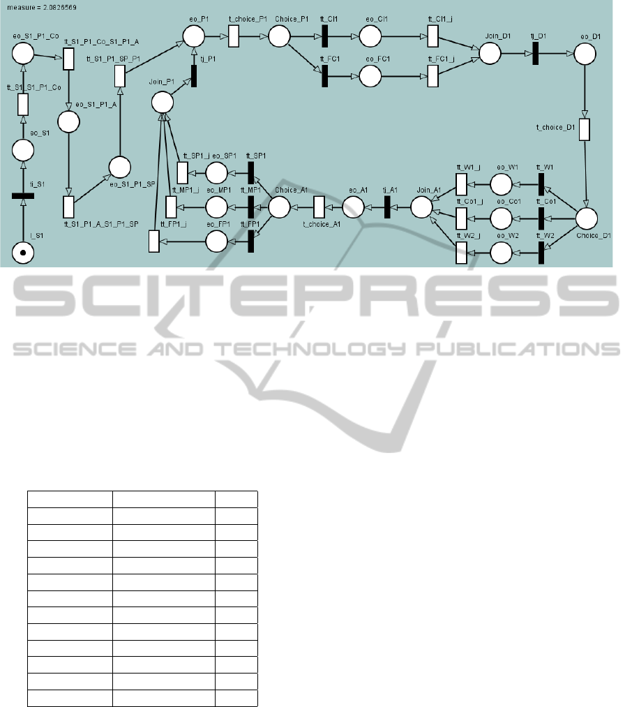
Figure 5: Resulting Petri net of the system.

the most power efﬁcient, statistically it can be used

only in 20% of cases. 3 out of 10 units are produced

in the middle-speed mode (MidProd1), and the half

of all orders must be done while using both reserve

motors (FastProd1). The component is then being

packed (Packaging1) and the production cycle is here

looped. The element Import states the XML ﬁle con-

taining operational model linked to the current appli-

cation model. An overview of the attributes given to

the states is summarized in the Table 3.

Table 3: Attributes stated in the application model.

State name execTime, min. prob

Start1

Packaging1

Cleaning1 0.9

FullClean1 0.1

Drying1

Waiting1 1 0.2

Continue1 0.7

Waiting2 5 0.1

Adaptation1

SlowProd1 0.2

MidProd1 0.3

FastProd1 0.5

To transform both models into SPN, the user

clicks eSMapp → eSMapp to eDSPN. The informa-

tion from the application model is being analyzed and

the missing data is taken from the operational model.

Thus, the power consumption is given only in the op-

erational model. For the states, where execution time

is not deﬁned in the application model, this value is

also taken from the operational model (e.g. Start1,

Packaging1, Cleaning1 and so on). Missing states be-

tween two similar states are added to make the tran-

sition stated in the application model possible (e.g.

states Continue, Adaptation and SlowProd are missed

between the states Start1 and Packaging1). The pa-

rameter delay of the exponential transitions is ﬁlled

up with the information from the attribute execTime

of the respective simple states. The formula for es-

timating the power consumption is being ﬁlled using

the information from the attribute powerPeak. The re-

sulting Petri net is shown in Fig. 5.

The stationary analysis of the Petri net results

that the power consumption of the system is equal to

2.0826569 Watt.

5 CONCLUSIONS

This paper presented an extension of the software

tool TimeNET for model-based estimation of power

consumption of embedded systems. The main con-

tribution of the paper is description of two new net

classes implemented in TimeNET for modeling the

system under consideration. UML extended with sev-

eral stereotypes of MARTE proﬁle is used for the

modeling process. For the modeling part, a system

is described with operational and application models,

which reﬂect correspondingly hardware and software

parts of the system. These two models are converted

automatically into a stochastic Petri net, which is then

used for the performance evaluation. The station-

ary analysis implemented in TimeNET lets the user

estimate power consumption of the whole system.

The application example an industrial control sys-

tem, demonstrating that the method is not restricted

to microcontroller-based embedded systems.

SIMULTECH2014-4thInternationalConferenceonSimulationandModelingMethodologies,Technologiesand

Applications

ACKNOWLEDGEMENTS

The authors would like to thank the Thuringian Min-

istry of Education, Science and Culture and the Ger-

man Academic Exchange Service (DAAD) for the ﬁ-

nancial support of the project. We also recognize the

valuable contribution of Andres Canabal Lavista and

his student working group to the software tool devel-

opment.

REFERENCES

Andrade, E., Maciel, P., Falc

ao, T., Nogueira, B., Araujo,

C., and Callou, G. (2009). Performance and energy

consumption estimation for commercial off-the-shelf

component system design. Innovations in Systems and

Software Engineering, 6(1-2):107–114.

Callou, G. R. d. A., Maciel, P. R. M., de Andrade, E. C.,

Nogueira, B. C. e. S., and Tavares, E. A. G. a. (2008).

A coloured petri net based approach for estimating ex-

ecution time and energy consumption in embedded

systems. In Proceedings of the 21st Annual Sym-

posium on Integrated Circuits and System Design,

SBCCI ’08, pages 134–139, New York, NY, USA.

ACM.

Dijkstra, E. (1959). A note on two problems in connexion

with graphs. Numerische Mathematik, 1(1):269–271.

German, R. (2000). Performance Analysis of Communica-

tion Systems, Modeling with Non-Markovian Stochas-

tic Petri Nets. John Wiley and Sons.

German, R., Kelling, C., Zimmermann, A., and Hommel,

G. (1995). TimeNET – a toolkit for evaluating non-

Markovian stochastic Petri nets. J. Performance Eval-

uation, 24:69–87.

Jakop, F. (2003). PENG – Plattformunabh

angiger Editor f

NetzGraphen. Master’s thesis, TU Berlin.

Jensen, K., Kristensen, K. L., and Wells, L. (2007).

Coloured Petri nets and CPN tools for modelling and

validation of concurrent systems. Int. Journal on

Software Tools for Technology Transfer (STTT), 9(3–

4):213–254.

Object Management Group (OMG) (2005). UML Proﬁle

for Schedulability, Performance, and Time Speciﬁca-

tion, Version 1.1.

Object Management Group (OMG) (2011). UML Proﬁle

for MARTE: Modeling and Analysis of Real-Time

Embedded Systems, Version 1.1.

Object Management Group (OMG) (2012). OMG Uni-

ﬁed Modeling Language (OMG UML), Infrastructure,

Version 2.4.1.

Shorin, D. and Zimmermann, A. (2013). Evaluation of Em-

bedded System Energy Usage with Extended UML

Models. In 2nd Workshop Energy Aware Software-

Engineering and Development (EASED@BUIS),

Softwaretechnik-Trends, 33(2), Oldenburg, Germany.

Shorin, D., Zimmermann, A., and Maciel, P. (2012). Trans-

forming UML State Machines into Stochastic Petri

Nets for Energy Consumption Estimation of Embed-

ded Systems. In 2nd IFIP Conference on Sustainable

Internet and ICT for Sustainability (SustainIT 2012),

Pisa, Italy.

Trowitzsch, J. (2007). Quantitative Evaluation of UML

State Machines Using Stochastic Petri Nets. PhD the-

sis, TU Berlin.

Trowitzsch, J., Jerzynek, D., and Zimmermann, A. (2007).

A Toolkit for Performability Evaluation Based on

Stochastic UML State Machines. In Proceedings

of the 2nd International Conference on Performance

Evaluation Methodologies and Tools (ValueTools),

Nantes, France.

Trowitzsch, J. and Zimmermann, A. (2005). Towards Quan-

titative Analysis of Real-Time UML Using Stochastic

Petri Nets. In Proceedings of the 13th International

Workshop on Parallel and Distibuted Real-Time Sys-

tems, Denver, Colorado. IEEE.

Zimmermann, A. (2012). Modeling and Evaluation of

Stochastic Petri Nets with TimeNET 4.1. In Proceed-

ings of the 6th International Conference on Perfor-

mance Evaluation Methodologies and Tools (Value-

Tools), pages 54–63. IEEE.

Zimmermann, A. and Hommel, G. (1999). Modelling and

evaluation of manufacturing systems using dedicated

Petri nets. Int. Journal of Advanced Manufacturing

Technology, 15:132–137.

ExtendingtheSoftwareToolTimeNETbyPowerConsumptionEstimationofUMLMARTEModels