Traditional vs Agile Development

A Comparison Using Chaos Theory

Doaa M. Shawky

Engineering Mathematics Department, Faculty of Engineering, Cairo University, Giza 12613, Egypt

Keywords: Agile Development, Waterfall Method, Software Metrics, Chaos Theory.

Abstract: Agile software development describes those methods with iterative and incremental development. This

development method came into view to overcome the drawbacks of traditional development methods.

Although agile development methods have become very popular since the introduction of the Agile

Manifesto in 2001, however, there is an ongoing debate about the strengths and weakness of these methods

in comparison with traditional ones. In this paper, a new dimension for the comparison between the two

methods is presented. We postulate that, since both methods are based mainly on human activity, the two

methods can be modeled using Chaos Theory. Source codes that are produced by the two methods in

subsequent versions are characterized by a set of software metrics. Modeling and analysis of these metrics

are performed using the Chaos Theory. Initial results show that the metrics sequences of both methods are

chaotic sequences. Furthermore, agile methods produce more chaotic metrics sequences. However, is being

chaotic a good or a bad feature? We argue that sometimes being chaotic is not a weakness, on the contrary,

it is a strength.

1 INTRODUCTION

Since the invention of the traditional waterfall

method by Royce in 1970 (Sommerville, 1996), it

has been used as a de facto standard for software

development processes. It is often described as the

stereotypical traditional method. Using this method,

the software development lifecycle is divided into

seven sequential stages: Conception, Initiation,

Analysis, Design, Construction, Testing, and

Maintenance. Traditional waterfall software

development approaches are usually considered

incapable of handling the development complexity

(Highsmith, 2013). Since the software industry,

software technology, and customers’ expectations

were moving very quickly and the customers were

becoming increasingly less able to fully state their

needs up front. As a result, agile methodologies and

practices emerged as an explicit attempt to more

formally embrace higher rates of requirements

change. Thus, in the past few years, agile software

development has emerged as a promising

methodology to complexity. Various agile

approaches have been proposed. Among the

methods which have gained a lot of popularity, the

eXtreme Programming (XP) (Beck and Andres,

2004) and Scrum (Schwaber and Beedle, 2002).

There is an ongoing debate about agile and

traditional methods and usually they are considered

opposition to each other. The waterfall model is

especially used for large and complex engineering

projects. However, it has some drawbacks, like

inflexibility in the face of changing requirements

(Sommerville and Kotonya, 1998), where the

requirements design absorbs a large amount of

project resources. In addition, well documentation is

necessary in all phases of the project life cycle. On

the other hand, agile methods deal well with

unstable and volatile requirements by employing

short iterations, early testing, and customer

collaboration (Martin, 2003). These characteristics

enable agile methods to deliver business value early

and improve it continuously throughout the life of

the project (Larman, 2003). In (Huo et al., 2004), the

authors conducted a study to compare between agile

and waterfall methods using software quality

assurance (QA) practices. They mentioned that in

agile methods, static and dynamic quality assurance

practices are combined in the short iterative phases

of the life cycle. Meanwhile in waterfall methods,

only static QA practices are possible in the analysis

109

Shawky D..

Traditional vs Agile Development - A Comparison Using Chaos Theory.

DOI: 10.5220/0005096501090114

In Proceedings of the 9th International Conference on Software Paradigm Trends (ICSOFT-PT-2014), pages 109-114

ISBN: 978-989-758-037-6

 2014 SCITEPRESS (Science and Technology Publications, Lda.)

phase. On the other hand, dynamic QA are used in

the Test phase, and they are combined in the Design

and Implementation phases. However, they

concluded that it is very difficult to compare the

software quality resulting from the two approaches

as they have different initial development

conditions.

Chaos refers to systems which are at an

intermediate point between the completely

predictable and the totally random ones. Examples

of chaotic systems in nature include tornadoes, stock

markets, turbulences, and weather (Casdagli, 1989).

Chaos theory is the one that deals with such systems.

At the heart of chaos theory is the notion that

complex systems can often be characterized by fairly

simple mathematical equations (Mandel, 1995).

The Chaos model and Chaos life cycle can be

used to define a concise framework for exploring,

interpreting, and assessing software development. In

this context, only few studies were found. For

instance, Wang et al. (Wang and Vidgen, 2007) have

analyzed the roles of structuring and planning in the

software development process using edge of chaos

concept from complex adaptive systems theory.

They have performed empirical studies of two

software development teams in the same IT

company where one of them is developed using an

agile methodology, XP, and the other using the

waterfall approach. Both software development

processes are analyzed using the “edge of chaos”

from the complex adaptive system theory. The

authors found that structuring and planning are

essential to agile processes and take different forms

from the waterfall model. In addition, they

concluded that the prescribed structures of the

waterfall method makes it chaotic. Also in (Wang

and Vidgen, 2007), the authors have proposed a

framework for the study of agile approaches using

complex adaptive system theory (CAS). Several

agile practices have been identified and linked to the

relevant CAS principles. The CAS framework was

applied to a case study that used XP. A strong

correspondence between CAS theory and the

practice of agile approaches was found. Moreover,

Raccoon (Raccoon, 1995) has used the principles of

chaos to study the relationships between a line of

code and the entire project. The author described the

development process from a developer’s point of

view. He used the Chaos model that combines a

linear problem solving loop with fractals to describe

the complexity of software development. Using

chaos theory, a linear problem-solving loop is

combined with fractals to suggest that a project

consists of many interrelated levels of problem

solving. In addition, the chaos model shows how

users, developers, and technologies interact during a

project. Although these works have provided a

framework that maps some agile principles to Chaos

theory, none of these works show how to apply the

power of Chaos theory in analysing the final product

of this chaotic process which is the source code

itself.

A software metric is a measure that generates a

numerical value for a piece or a specification of the

software (Cem Kaner, 2013). Some common metrics

include source lines of code (SLOC), cyclomatic

complexity, Function Point Analysis (FPA), etc.

Previously, we have used software metrics in re-

engineering and maintenance activities (Shawky,

2008a, Shawky, 2008b), clone detection (Shawky

and Ali, 2010b, Shawky and Ali, 2010c) and in

defining a measure for software agility (Shawky and

Ali, 2010a). In this paper, the final product of a

software development process which is the source

code, is characterized by a set of software metrics.

The subsequent versions of analyzed systems are

characterized by a set of software metrics. These

sequences of values are then analyzed and modelled

by the Chaos Theory. This analysis allows for

prediction or forecasting of the system’s behaviour

in the near future (Tsoukas, 1998).

In the first step of the proposed approach, we

statically scan implementation files using the static

analysis and metrics generation tool Understand

(www.scitools.com). Although we used only the two

metrics SLOC and Cyclomatic Complexity which

both can be used to represent the complexity

characteristics of the analyzed system, however, the

analysis can be extended to include other metrics. In

the second step, we analyzed the two sequences that

were generated for the two metrics in the subsequent

versions of the studied systems. Chaos theory is used

in modelling and analysing these sequences.

Obtained results show that both sequences are

chaotic and that the sequence of metrics values for

the system that was developed using agile methods

is more “chaotic” than the other sequence.

The rest of this paper is organized as follows.

Section 2 presents a background on Chaos Theory.

In Section 3, the proposed approach is presented in

detail. Section 4 summarizes the results. Finally

Section 5 introduces conclusions and future work.

2 CHAOS THEORY

Chaos is a property of some deterministic systems.

A deterministic system is one in which future states

depend on the current conditions. They can be

ICSOFT-PT2014-9thInternationalConferenceonSoftwareParadigmTrends

110

modelled by dynamical systems. Historically the

idea has been that all processes occurring in the

universe are deterministic, and that if we knew

enough of the rules governing the behaviour of the

universe and had measurements about its current

state we could predict what would happen in the

future.

Chaotic systems must have some characteristics

(Mandel, 1995, Wang et al., 2008). These include

the following. Most complex systems exhibit what is

called attractors which are the states or patterns the

system eventually settles into. Some systems tend

toward traditional fixed points or limit cycles. On

the other hand, chaotic systems have strange

attractors which are unrepeated patterns. Also, long-

term prediction is mostly impossible due to

sensitivity to initial conditions. The lack of long-

term predictability in chaotic systems does not imply

that short-term prediction is impossible. In

counterpoint to purely random systems, chaotic

systems can be predicted for a short interval into the

future.

The first step in the analysis of a chaotic time

series data was introduced in (Packard et al., 1980)

in which state-space reconstruction of time series

data was proposed for the first time. The

mathematical justification of this approach was

presented in (Takens, 1981) where the reconstructed

state space is proved to be one-to-one equivalent to

the original state space of the real-life system. The

reconstruction of state space can be summarized as

follows: Given s (t); a scalar function describing the

system, sampled at time interval τ

, and starting at

some time t0, the nth sample can be represented as:

= s (t

+ (n − 1) τ

), n = 1, 2, . . . (1)

A delay-coordinate reconstruction can be formed

by plotting the time series versus one or more time-

delayed version(s) of it. For a 2-dimensional

reconstruction, we plot the delay vector y(n) = [s

−L ], n =L +1, L +2, . . ., where L is the lag or

sampling delay, i.e., the difference between the

adjacent components of the delay vector in number

of samples. For a d-dimensional reconstruction, the

delay vector, y(n) can be written as given by (2):

y(n) = [s

, s

n−L

, · · · , s

n−(d−2)L

, s

n−(d−1)L

] (2)

It was proved by Taken’s theory (Takens, 1981)

that if d is large enough, the vector series y(n)

reproduces many of the important dynamical

characteristics of the original series. Thus, one does

not need the original vector series in order to analyze

many of the system properties of the data series.

Specifically, if the dimension of the reconstructed

space, d, is larger than twice m which is the number

of active degrees of freedom, the equivalence of the

spaces is guaranteed. From a mathematical point of

view, the selection of L has no effect on the

embedding of a noise-free time series. However, in

practical applications and for data contaminated with

noise, a good choice of L has an important impact on

the analysis (Casdagli et al., 1991). If L is too small

in comparison with the dynamic variation of the

system, successive elements of the delay vectors are

strongly correlated. If L is too large, successive

elements are almost independent. In delay-

coordinate reconstruction, the selection of time delay

and dimension are the most important issues (Fraser

and Swinney, 1986). For the calculation of time lag,

different approaches are proposed in the literature

(Fraser and Swinney, 1986, Shinbrot et al.,

1993).Among them, the autocorrelation function and

mutual information approach are the most general

and common. In our approach, we will use the

mutual information method which can account for

any nonlinear dynamical correlation in contrast to

the use of the autocorrelation function (Shinbrot et

al., 1993).

The mutual information for sampling delay L

can be defined as:

I (L) =

∑

Ps





log





,

















(3)

where P









is the probability that the signal

has a value in the histogram representing the mutual

information function. Informally, this function

quantifies the information that we have about s

n+L

given that we know sn. Usually, the sampling lag

related to the first minimum of the mutual

information function specifies the point where the

information about s

n+L

given knowledge of s

or the

redundancy has a local minimum.

Another important concept in chaos theory is the

fractal dimension. Fractal dimensions quantify the

self-similarity of a geometrical object (Liebert and

Schuster, 1989). One of the most used dimensions is

the correlation dimension which is non integer for

chaotic data indicating the presence of strange

attractors. It can be calculated using correlation

integral, which is an estimate of the probability that

two points on the attractor lay less than a distance R

from each other. Given the N values of the series

and for fixed embedding dimension d and time lag L

, we calculate the percentage of points within a

certain distance R from one another, for increasing

values of R, through the correlation integral (C(R)).

As proposed in (Hilborn, 2000), C(R) can be

calculated as given by (4) for a fixed time lag L:











∑∑

HR 

‖





yj

‖





,





(4)

Where H(x) is the Heaviside step function with

H(x) =1 for x>0, and H(x) =0 for x≤0. A log/log

TraditionalvsAgileDevelopment-AComparisonUsingChaosTheory

111

plot of the output and an estimate of the slope of the

linear region of this graph gives the correlation

dimension dc due to the fact that, by increasing the

value of R, C(R) should increase as R

, or, after

taking the logarithm of both sides, Log (C(R)) = dc

Log (R) + constant. We repeat these calculations for

increasing values of embedding dimensions d while

keeping the value of the time lag L fixed. The value

of dc should eventually converge, by increasing d, to

the true value of the fractal dimension of the

attractor. Usually, the proper embedding dimension

must be an integer greater than or equal to twice d

plus one (Hilborn, 2000).

A common method for the identification of

chaos in state-space systems is to calculate the

largest Lyapunov exponent (LLE) (Shinbrot et al.,

1993, Mandel, 1995). The calculation of this

exponent from time series data has been extensively

considered in the literature (Ramasubramanian and

Sriram, 2000). Lyapunov exponents represent the

average exponential rates of divergence or

convergence of nearby orbits in phase space

(Shinbrot et al., 1993). Any system containing at

least one positive Lyapunov exponent is defined to

be chaotic, with the magnitude of the exponent

reflecting the time scale on which system dynamics

become unpredictable (Wolf et al., 1985). To

calculate Lyapunov exponent, a step by step

evolution of a pair of points, a reference one and a

candidate one is done. Each time the distance

between these two points becomes too long, a

replacement procedure of the candidate is applied in

such a way that the orientation between the new pair

of points is as close as possible to that of the original

pair. The details of the used algorithm for

calculating Lyapunov exponent can be found in

(Wolf et al., 1985). Another method for detecting the

presence of chaos is the calculation of correlation

dimension as given in (4). The non-integer value

indicates the existence of chaos (Packard et al.,

1980).

3 AN EXPERIMENTAL STUDY

3.1 Subject Systems

To evaluate our approach we used as case studies

two open source systems. The first one is FileZilla

(http://filezilla-project.org/) which is an open source,

cross-platform, and FTP client. This system was

developed using traditional methods. The second

system is Suneido (http://sourceforge.net/

projects/suneido/) which is an open source system

for developing and deploying applications across

networks using an object-oriented programming

language IDE. Both systems are written in C++. We

used 20 subsequent versions of each system. The

used versions of FileZilla have the time span from 3-

11-2004 to 30-11-2007. Meanwhile, the used

versions of Suneido cover the time span from 29-9-

2001 to 28-10-2007.

3.2 Experimental Analysis

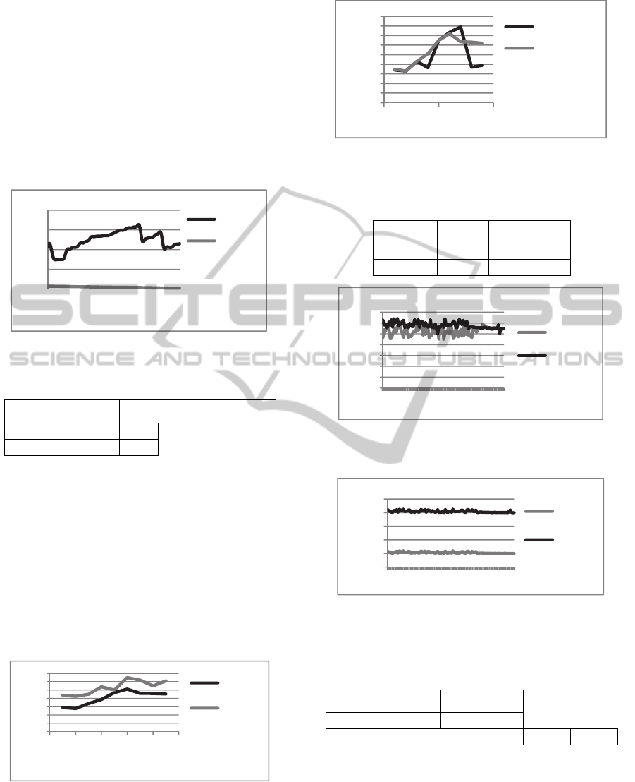
Figures 1 and 2 show the SLOC and Complexity

values in the two sequences for FileZilla and

Suneido respectively. Before starting the modelling

process, we interpolated the sequences of metrics

values for the two systems. This step is necessary for

sampling more data points to make the next analysis

steps feasible. For instance, Figure 3 shows the

interpolated time series for FileZilla. The time step

is calculated as the difference between the release

date of the last and the first version studied divided

by the number of points. Thus it was set to 1.4 day

(4x12x30/1000) approximately

Figure 1: SLOC Sequences for the two systems.

Figure 2: Complexity Sequences for the two systems.

Mutual information is calculated for each set of

data points using (3). The first minimum of mutual

information is used to determine the optimal time

delays. Table 1 indicates the calculated optimum

time delays for each data set.

We then calculate the correlation dimension for

each of the used datasets. Then using (4), we

calculated logC(R) and log(R) for different

100

150

0 5 10 15 20

KSLOC

FileZilla

KSLOC

Suneido

KSLOC

01020

Cyclomatic Complexity

FileZilla

Complexity

Suneido

Complexity

ICSOFT-PT2014-9thInternationalConferenceonSoftwareParadigmTrends

112

embedding dimensions d ranging from 1 to 10 for

the four sequences. The slope of the linear part

approximates dc. Figure 4 and Figure 5 show the

correlation dimension (dc) vs. the embedding

dimension (d) for the used sequences. It should be

mentioned that as d increases dc saturates at a non-

integer value (ds) which indicates chaos. Correlation

dimensions for the used sequences are presented in

Table 2. As shown in the table, correlation

dimensions are non-integers which also indicates

chaos.

Figure 3: Interpolated time series for FileZilla.

Table 1: Time delays for the used systems.

Syste

SLOC Complexity

FileZilla 29 21

Suneido 33 28

Another indication of chaos is the positive LLE.

Figure 6 and Figure 7 show that LLE’s for SLOC

and Complexity sequences of the two systems are

positive. Meanwhile, Table 3 represents the final

value of LLE’s for the four sequences which are the

saturated LLE’s in Figure 6 and 7. As shown in the

table, Suneido’s sequences have larger LLE’s

values. This indicates that the source code and

complexity of Suneido are less predictable than

FileZilla and that it has a larger rate of information

change than that of FileZilla.

Figure 4: Correlation dimension (dc) vs. embedding

dimension (d) for SLOC sequences.

Figure 5: Correlation dimension (dc) vs. embedding

dimension (d) for Complexity sequences.

Table 2: Correlation dimensions for the used systems.

Syste

SLOC Complexity

FileZilla 1.62 1.19

Suneido 1.86 1.41

Figure 6: Largest Lyaponuv exponent (LLE) for SLOC

sequences.

Figure 7: Largest Lyaponuv exponent (LLE) for

Complexity sequences.

Table 3: Largest Lyapunov Exponents for the used

systems.

Syste

SLOC Complexity

FileZilla 0.455 0.10

Suneido 0.457 0.13

4 CONCLUSIONS

This paper presents a comparison between agile and

waterfall development methods using the Chaos

Theory. Two open source systems that were

developed using the two development methods are

100

150

200

1 201 401 601 801

Time steps ( x 1.4 day)

SLOC

Complexity

0,8

1,2

1,4

1,6

1,8

2,2

0246810

Embedding dimension (d)

FileZilla

SLOC

Suniedo

SLOC

0,8

0,9

1,1

1,2

1,3

1,4

1,5

1,6

1,7

0510

Embedding dimension (d)

FileZella

Complexity

Suneido

Complexity

0,4

0,41

0,42

0,43

0,44

0,45

0,46

0,47

LLE

Time Steps

FileZilla

KSLOC

Suneido

KSLOC

0,09

0,1

0,11

0,12

0,13

0,14

LLE

Time Step

FileZilla

Complexity

Suneido

Complextiy

TraditionalvsAgileDevelopment-AComparisonUsingChaosTheory

113

used as case studies. The analyses of subsequent

versions of the two systems show that both systems

have chaos. Furthermore, the system developed

using agile methods is more chaotic than the one that

was developed using traditional methods. Although

being chaotic has several drawbacks, for instance,

complex undetermined behaviour and high

sensitivity to changes in initial conditions, however,

a chaotic system has many advantages e.g.,

flexibility, creativity and stability. In addition, for

chaotic systems with large LLE, a quick settlement

to the steady state is expected. Thus, agile

development results in a more chaotic system with

varying and constantly changing elements that settle

down more quickly than those developed using

waterfall methods.

As a future work, more systems need to be

analyzed to be able to generalize the findings.

Another set of interesting questions include the

following. What quality attributes of the software

are more chaotic when agile methods are used?

What agile

approaches produce more chaotic

systems, and why?

REFERENCES

Beck, K. & Andres, C. 2004. Extreme Programming

Explained: Embrace Change, Addison-Wesley

Professional.

Casdagli, M. 1989. Nonlinear Prediction Of Chaotic Time

Series. Physica D: Nonlinear Phenomena, 35,335-356.

Casdagli, M., Eubank, S., Farmer, J. D. & Gibson, J. 1991.

State Space Reconstruction In The Presence Of Noise.

Physica D: Nonlinear Phenomena, 51, 52-98.

Cem Kaner, S. M., Walter P. Bond. Software Engineering

Metrics: What Do They Measure And How Do We

Know? In Metrics 2004. Ieee Cs, 2013.

Fraser, A. M. & Swinney, H. L. 1986. Independent

Coordinates For Strange Attractors From Mutual

Information. Physical Review A, 33, 1134.

Highsmith, J. 2013. Adaptive Software Development: A

Collaborative Approach To Managing Complex

Systems, Addison-Wesley.

Hilborn, R. C. 2000. Chaos And Nonlinear Dynamics: An

Introduction For Scientists And Engineers, Oxford

University Press.

Huo, M., Verner, J., Zhu, L. & Babar, M. A. Software

Quality And Agile Methods. Computer Software And

Applications Conference, 2004. Compsac 2004.

Proceedings Of The 28th Annual International, 2004.

Ieee, 520-525.

Larman, C. 2003. Agile And Iterative Development: A

Manager's Guide, Addison-Wesley Professional.

Liebert, W. & Schuster, H. 1989. Proper Choice Of The

Time Delay For The Analysis Of Chaotic Time Series.

Physics Letters A, 142, 107-111.

Mandel, D. R. 1995. Chaos Theory, Sensitive Dependence,

And The Logistic Equation.

Martin, R. C. 2003. Agile Software Development:

Principles, Patterns, And Practices, Prentice Hall Ptr.

Packard, N., Crutchfield, J., Farmer, J. & Shaw, R. 1980.

Geometry From A Time Series.

Raccoon, L. 1995. The Chaos Model and The Chaos Cycle.

Acm Sigsoft Software Engineering Notes, 20, 55-66.

Ramasubramanian, K. & Sriram, M. 2000. A Comparative

Study Of Computation Of Lyapunov Spectra With

Different Algorithms. Physica D: Nonlinear

Phenomena, 139, 72-86.

Schwaber, K. & Beedle, M. 2002. Gilè Software

Development With Scrum.

Shawky, D. M. 2008a. The Application Of Rough Sets

Theory As A Tool For Analyzing Dynamically

Collected Data. Journal Of Engineering And Applied

Science, 55, 473-490.

Shawky, D. M. 2008b. Towards Locating Features Using

Digital Signal Processing Techniques. Journal Of

Engineering And Applied Science, 50, 1-20.

Shawky, D. M. & Ali, A. F. A Practical Measure For The

Agility Of Software Development Processes. Computer

Technology And Development (ICCTD), 2010 2nd

International Conference On, 2-4 Nov. 2010 2010a.

230-234.

Shawky, D. M. & Ali, A. F. An Approach For Assessing

Similarity Metrics Used In Metric-Based Clone

Detection Techniques. Computer Science And

Information Technology (ICCSIT), 2010 3rd IEEE

International Conference On, 9-11 July 2010 2010b.

580-584.

Shawky, D. M. & Ali, A. F. Modeling Clones Evolution In

Open Source Systems Through Chaos Theory.

Software Technology And Engineering (Icste), 2010

2nd International Conference On, 3-5 Oct. 2010 2010c.

V1-159-V1-164.

Shinbrot, T., Grebogi, C., Ott, E. & Yorke, J. A. 1993.

Using Small Perturbations To Control Chaos. Nature,

363, 411-417.

Sommerville, I. 1996. Software Process Models. Acm

Computing Surveys (Csur), 28, 269-271.

Sommerville, I. & Kotonya, G. 1998. Requirements

Engineering: Processes And Techniques, John Wiley &

Sons, Inc.

Takens, F. 1981. Detecting Strange Attractors In

Turbulence. Dynamical Systems And Turbulence,

Warwick 1980. Springer.

Tsoukas, H. 1998. Introduction: Chaos, Complexity And

Organization Theory. Organization, 5, 291-313.

Wang, L. & Vidgen, R. 2007. Order and Chaos In Software

Development: A Comparison of Two Software

Development Teams In a Major It Company.

Wang, L., Xing, X. & Chu, Z. On Definitions Of Chaos In

Discrete Dynamical System. Young Computer

Scientists, 2008. Icycs 2008. The 9th International

Conference for, 2008. Ieee, 2874-2878.

Wolf, A., Swift, J. B., Swinney, H. L. & Vastano, J. A.

1985. Determining Lyapunov Exponents From A Time

Series. Physica D: Nonlinear Phenomena, 16, 285-317.

ICSOFT-PT2014-9thInternationalConferenceonSoftwareParadigmTrends

114