Cycle-to-Cycle Transient Model of 4-stroke Combustion Engines

Madan Kumar and Tielong Shen

Department of Engineering and Applied Science, Sophia University, Tokyo, Japan

Keywords:

Modeling, Combustion Engines, Discrete-time System.

Abstract:

In 4-stroke combustion engines, managing the cycle-to-cycle transient characteristics of the mass of the air,

the fuel and the burnt gas is an important issue due to the cycle-to-cycle coupling caused by the imbalance

of cyclic combustion. This paper presents a discrete-time model that represents the cycle-to-cycle transient

behavior of in-cylinder state variables under the assumption of measurability of the total gas mass and the

residual gas fraction. It is shown that if the state variables are chosen as total fuel mass, residual unburnt

air and the burnt gas mass, then the system is modeled as a time-varying linear system. Validation results is

demonstrated which conducted on a full-scaled gasoline engine test bench.

1 INTRODUCTION

In internal combustion engine, combustion inside the

cylinder is a complex phenomena and exhibit sub-

stantial cycle-to-cycle variation. This cyclic variation

is observed to stochastic in process. Some physical

model has been developed to characterized the tran-

sient behavior of engine phenomena on cycle basis

[(Rizzoni, 1989),(Peyton Jones, 2010)]. This cyclic

variation affects the engine performance, such as air-

fuel ratio, torque generation and so on. The mainly

affecting variables are residual gas, unburned fuel and

unburned air succeeding the next cycle from previous

cycle. There are so many factors that inﬂuence the

cyclic residual gas, and it is not feasible to represent

the inﬂuence mathematically in general. Analysis and

research in this area is continue from 19th century

(Clerk,1886) and still there is some gap in satisfactory

solution. In engine research’s, researchers mainly aim

to improve the power generation and reduce the emis-

sion due to the limitation of sources of fuel and envi-

ronmental pollution effect. The engine performance

goes down with the increases of residual gas in en-

gine cylinder. However it decreases the emission as

NOx decreases in cylinder due to in-cylinder temper-

ature decreases.

On another side, a good modeling mechanism of

the engine is also a fact to improve the performance

of engine. Since the in-cylinder phenomena like in-

cylinder air, fuel and residual gas compositions are

not measurable directly except to in cylinder pressure,

model based observers are thus necessary to estimate

these quantities. This ambiguity has created a con-

tinuing challenging to ﬁnd a suitable control model

to estimate the true nature of in-cylinder cycle-to-

cycle behavior [(Daw, 1996),(Daw, 1998),(Jonathan,

2008),(Yang, 2013)].

In this paper a discrete-time model that represents

the cycle-to-cycle transient behavior of in-cylinder

state variables under the assumption of measurabil-

ity of the total gas mass and the residual gas fraction

is proposed. The system is modeled as a time-varying

linear system as the state variables are chosen as to-

tal fuel mass, residual unburnt air and the burnt gas

mass.Validation results are demonstrated which con-

ducted on a full-scaled gasoline engine test bench.

The detail about the evaluation of total charge and

residual gas fraction are discussed in next section.

2 SYSTEM DESCRIPTIONS

As is well known that the in-cylinder gas and com-

bustion phenomena are difﬁcult to measured directly

on cycle-to-cycle basis in engine dynamic systems. In

internal combustion engines, fuel and air goes inside

the engine cylinder and releases heat energy due to

the chemical reaction happened between fuel and air

and this heat energy is used to convert in mechanical

energy to produced the work. In four strokes engine,

one cycle includes the suction, compression, combus-

tion and exhaust process. In general, fresh air and

fuel mixture enters in cylinder during suction stroke

and it compressed during compression in four stroke

745

Kumar M. and Shen T..

Cycle-to-Cycle Transient Model of 4-stroke Combustion Engines.

DOI: 10.5220/0005095107450750

In Proceedings of the 4th International Conference on Simulation and Modeling Methodologies, Technologies and Applications (SIMULTECH-2014),

pages 745-750

ISBN: 978-989-758-038-3

 2014 SCITEPRESS (Science and Technology Publications, Lda.)

gasoline engine. For the start of combustion, spark

is generated 30 to 40 deg. before top dead centre

(TDC) which depends upon the engine conﬁguration

and power required. In combustion stroke due to high

pressure and temperature inside the cylinder, piston

pushed out towards bottom dead centre (BDC) by the

in-cylinder high pressure and temperature charge and

hence power transfered to crank shaft. At the end of

combustion stroke, the exhaust valve open and ex-

haust gas expelled due to the high pressure of gas

inside the cylinder. In advance research, the direct

injection gasoline is used for improved the combus-

tion phenomena and performance of engines in which

gasoline is direct injected in port or in cylinder which

is named as gasoline direct injection (GDI) engine.

Due to the limitation in engine design, the exhaust

gas in one cycle does not expelled fully during the ex-

haust stroke and it remains for the next cycle which

affects the combustion in next cycle. The engine per-

formance is affected due to this remained gas in cylin-

der.

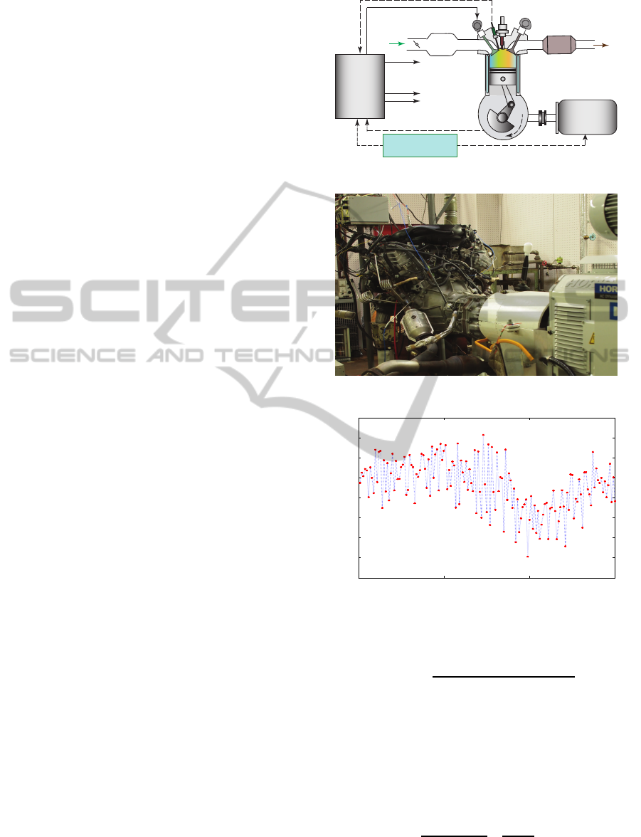
In engine, variable valve timing (VVT) system,

engine speed and load also affects the cycle to cy-

cle variation. A schematic diagram of experimental

setup with VVT control system is shown in Fig.1. A

gasoline 3.5L engine is used for the experiment which

is supported by Toyota Motors Corporation (Fig.2).

This engine having port and direct injection system

and engine is well instrumented to get almost full data

to analyze the engine behavior. In this engine, VVT

system is also in-build for the analysis of the effects

of VVT on in-cylinder gas contains during cycle-to-

cycle ﬂuctuation. For control and capturing the data,

ECU and dSPACE are used.

In this experimental test bench, experiment is con-

ducted for the measurement of total charge and resid-

ual gas estimation on the cycle basis keeping the ﬁxed

spark advance and torque and varying the VVT. The

variation in the magnitude of total charge and residual

gas is observed to ﬂuctuate on cycle to cycle basis. A

sample of variation in residual gas fraction (RGF) on

cycle basis is shown in Fig.3. From ﬁgure 3, it is ob-

served that the cyclic variation of residual gas fraction

is in stochastic process which cannot be predicted eas-

ily for the next cycle.

The total charge is calculated in compression

stroke before start of combustion and residual gas

fraction (RGF) at the end of exhaust stroke on cycle

to cycle basis. The total charge in-cylinder can be

calculated by two method. (a). Using the direct mea-

surement of fresh inducted air, fresh injected fuel and

estimated RGF using pressure sensor. (b). Using the

in-cylinder pressure data. The total charge estimated

by direct measurement of fresh inducted air, fuel in-

Exhaust Gas

6. Exhaust VVT

2. Intake Manifold

Air ow

5. Spark Plug

dSPACE

ECU

Dynamometer

Control Panel

3. Intake VVT

4. Pressure Sensor

1. Throttle

7. Ehxaust Muer

Dynamometer

Figure 1: Schematic diagram of experimental setup.

Figure 2: Engine Setup.

0 50 100 150

0.03

0.035

0.04

0.045

0.05

0.055

0.06

0.065

0.07

Cycle

RGF

Figure 3: Cyclic residual gas fraction (RGF) sample.

jected and RGF is as given below,

(k) =

ind

(k− 1) + m

(k− 1)

(1− r(k))

(1)

where m

ind

(k − 1) and m

(k − 1) are the fresh in-

ducted air charge and injected fuel respectively from

the previous cycle for the combustion of present cycle

on the basis of cycle deﬁnition as shown in Fig.5.

In the second method, total charge is calcu-

lated using the in-cylinder pressure data [(Arsie,

2013),(Desantes, 2010)] as given below,

(k) =

∆P(k)V

(k)

{(

(k)

)

− 1}

−1

(2)

where ∆P is the difference of pressure P

(k) and

(k).

SIMULTECH2014-4thInternationalConferenceonSimulationandModelingMethodologies,Technologiesand

Applications

746

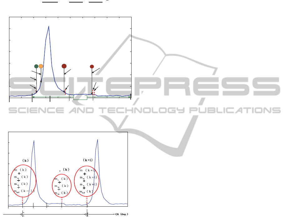
Similarly, the residual gas fraction r(k) at the end

of exhaust stroke can also be calculated using in-

cylinder pressure data as given in equation 3 (Yang,

2013). A ﬁgure for suitable measurement points for

pressure and volume is shown in Fig.4.

r(k) =

(k)

= (

(k)

)(

(k)

)

(3)

CA (deg.)

Cylinder Pressure

BDC

cycle

BDC

TDC

aIVC

IVC

(71

aBDC

)

EVO

(64

bBDC

)

bEVO

b TDC

EVC

aTDC

IVO

−3

bTDC

TDC

Figure 4: Pressure measurement points indication in pres-

sure vs crank angle plot.

Cylinder Pressure

BDC

TDC

BDC

TDC

K th cycle

TDC

K-1 th cycle K+1th cycle

CA㸦GHJ

㸧㸧

㹫

㸦㹩㸧

㸦㹩㸧

㹰

㸦㹩㸧

Figure 5: Gas exchange phenomena between cycle.

3 MODELING

For the development of model, cycle is deﬁned from

BDCi (k) to BDCi(k+1) as kth cycle in which data at

BDCi (k) is included in k

cycle and data at BDCi

(k+1) is included in k + 1

cycle as shown in Fig.5.

In this model, next cycle (k+ 1

cycle) variables can

be estimated using the present cycle (k

cycle) vari-

ables using the input control as fresh fuel injection

. From Fig.5, It can be observe that the total mass

of charge M

(k) including fresh charge of present cy-

cle and residual gas mass, unburned air and fuel mass

from previous cycle will be involved for the present

cycle combustion process. A cyclic representation of

gas exchange phenomena during cycle to cycle and in

cycle is shown in Fig.5.

According to cycle deﬁnition as shown in Fig.5

and with the assumptions of mass conservation during

the gas exchange in cycle to cycle process, the total

mass of fuel, mass of unreacted air (residual air) and

residual burned gas present for the combustion in k+

cycle is derived as,

a). The total mass of fuel available at the start of

combustion for k + 1

cycle is equal to the summa-

tion of mass of unreacted fuel in k

cycle and fresh

fuel injected in k

cycle as cycle deﬁnition. In math-

ematical form, the equation can be represented as,

(k+ 1) = m

fur

(k) + m

(k)

= (1−C

(k)(r(k))m

(k) + u

(k)

(4)

b). The unreacted air (residual air) at the start of

combustion in k+ 1

cycle is equal to the residual air

which is remained at the end of k

cycle and repre-

sented as,

(k+ 1) = r(k){ [m

(k) + m

ind

(k− 1)]

−λ

(k)m

(k)}

= r(k)m

(k)−λ

r(k)C

(k)m

(k)

+r(k)m

ina

(k− 1)

(5)

c). The burned gas at the start of combustion in k+1

cycle is equal to the residual burned gas at the end of

cycle and is represented as,

(k+ 1) = r(k)[m

(k) +C

(k)m

(k)

+λ

(k)m

(k)]

= r(k)m

(k)

+r(k)C

(k)(1+ λ

(k)

(6)

And total mass of charge M

(k) before start of

combustion in kth cycle assuming mass conservation

during process is as,

(k) = m

(k) + m

ind

(k− 1)

(7)

where, m

(k) is the total mass of fuel (= m

(k) +

fur

(k − 1)) available in the cylinder at the start

of combustion, m

fur

is unreacted fuel from pre-

vious cycle which is available for the combustion

in present cycle, C

is the combustion efﬁciency,

(k) = m

(k)) is fresh fuel injected, r(k) is resid-

ual gas fraction(RGF), m

is unreacted air mass, λ

is the stoichiometric air fuel ratio, m

ind

(k− 1) is fresh

air inducted in cylinder during suction stroke and m

is burned gas mass.

For the sake of simplicity, the assumptions for

(k) and r(k) variations for the simulation are con-

sidered as,

1). C

(k) = C

(1+σ(k)) = C

+ e(k),

e(k) ∈ N(0, σ

)

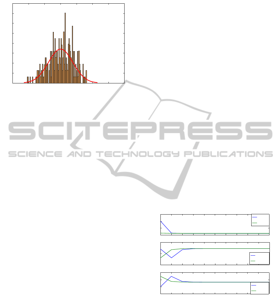
2). r(k) is measurable using equation 3 and a dis-

tribution sample is given in below Fig 6.

Cycle-to-CycleTransientModelof4-strokeCombustionEngines

747

0.04 0.045 0.05 0.055 0.06 0.065 0.07 0.075

100

150

200

250

300

350

400

r(k)

Probability

Figure 6: r(k) distribution sample.

where, e(k) is the variance of the distribution.

Equation number 4, 5 and 6 can be written in ma-

trix form as given below,





(k+ 1)









(1−C

(k))r(k) 0 0

−λ

r(k)C

(k) r(k) 0

r(k)C

(k)(1+ λ

) 0 r(k)









(k)













(k) +





r(k)





(∆+ ζ(k))

(8)

For the modeling and control systems, two assump-

tions are consider as follows,

1). m

ind

(k− 1) = ∆ + ζ(k)

2). y(k) = M

(k) − ∆

where, y(k) = Σx(k), ∆ is constant and assumed

to measurable (= m

ind

(k − 1)), ζ(k) is variance (

ζ(k) ∈ N(0, σ

Then ﬁnally from equation 8, the discrete time

model for estimation of cycle to cycle behaviors and

its control is represented as,

x(k+ 1) = A(k)x(k) + B

(k)

(k)(∆+ ζ(k))

(9)

mod

(k) = Cx(k) + ζ(k)

(10)

where x(k) is the state variables and A(k), B

(k),B

(k)

and C are constants as given below,

x(k) =





(k)





, C =



1 1 1



A(k) =





(1−C

(k))r(k) 0 0

−λ

r(k)C

(k) r(k) 0

r(k)C

(k)(1+ λ

) 0 r(k)













and B

(k) =





r(k)





4 VALIDATION

Validation of model is done on the static state using

ﬁxed input and variables and also on the actual ex-

perimental data. The inﬂuence of variables are also

found out in this section adding some noise in ﬁxed

input variables and parameters.

4.1 Simulation Results

In this case, initially ﬁxed input data is used for

the validation of model is as, C

(k) = 0.8 , r(k)

= 0.1, ∆ =15 mg, u

(k) = ∆/14.6 and x(0) =



1 1.5 0.8



Using the above initial input data in model, the

equilibrium points of initial value of x(0) are cal-

culated by simulation and thereafter this equilibrium

data is used as initial value of x(0) for further analysis.

0 0.1 0.2 0.3 0.4 0.5 0.6 0.7 0.8 0.9 1

1.0484

x 10

−6

(k)

(k+1)

0 0.1 0.2 0.3 0.4 0.5 0.6 0.7 0.8 0.9 1

3.0605

3.061

3.0615

x 10

−7

(k)

(k+1)

0 0.1 0.2 0.3 0.4 0.5 0.6 0.7 0.8 0.9 1

1.4537

1.4538

x 10

−6

Time (s)

(k)

(k+1)

Figure 7: x(k) and x(k+1).

A variation in state variables x(k) and x(k+ 1) are

shown in Fig.7. In this graph, it can be observe that

the both signals are able to merged after some delay

of time during simulation. The input signal C

(k) and

r(k) have added 20 percent noise in signal and also

input value of u

(k) is changed by magnitude of 15

percent for 10 second during the simulation time for

the observing the inﬂuence of fuel injection on x(k)

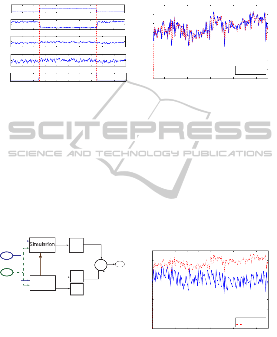
and y(k). The result is as shown in Fig.8. From ﬁgure,

it can be seen that due to changes of u

(k), m

(k)

SIMULTECH2014-4thInternationalConferenceonSimulationandModelingMethodologies,Technologiesand

Applications

748

0 2 4 6 8 10 12 14 16 18 20

1.2

1.4

x 10

−6

0 2 4 6 8 10 12 14 16 18 20

x 10

−7

0 2 4 6 8 10 12 14 16 18 20

x 10

−6

0 2 4 6 8 10 12 14 16 18 20

x 10

−6

mod

(k)

0 2 4 6 8 10 12 14 16 18 20

1.1

1.2

x 10

−6

Time (s)

(k)

Figure 8: Inﬂuence of u

(k) on x(k) and y(k).

and m

(k) are changes signiﬁcantly but there are less

inﬂuence on m

(k) and y

mod

(k) is noted.

4.2 Experimental Validation

For the model validation in realistic condition of en-

gine behavior, the experimental data of RGF and total

charge from engine experiment are used for simula-

tion. The value of y(k) calculated from the model and

from the engine data are compared in this section. A

block diagram of simulation is shown in Fig.9. From

the block diagram, it can be seen that the m

ind

and

are the input variables for the engine and simula-

tion both. From simulation, we can ﬁnd the value of

mod

(k) using the RGF data from the engine experi-

ment. On another side, the y

cal

(k) can also be calcu-

lated from the engine experimental data.

Simulation

ENGINE

ind

RGF

x(k)

(k)

equ-

(10)

equ-

(11)

equ-

(12)

cal

(k)

mod

(k)

Error

Figure 9: Block diagram of simulation.

4.2.1 Validation using M

(k)

In this case, y

cal

(k) is calculated using the below

given formula and compared with the y

mod

(k) model,

cal

(k) = M

(k) − ∆

(11)

where M

(k) can be calculated using equation (1) and

∆ can be measured by sensor. A comparison graph of

cal

(k) and y

mod

(k) is shown in Fig.10. From graph

0 2 4 6 8 10 12 14 16 18 20

1.05

1.1

1.15

1.2

1.25

1.3

1.35

1.4

x 10

−4

Time (s)

y(k)

cal

using M

mod

(k) using model

Figure 10: y

cal

(k) and y

mod

(k).

it can be observed that the y

cal

(k) and y

mod

(k) are ap-

proximately equal after some delay of simulation cy-

cle.

4.2.2 Validation using M

(k)

In this case, y

cal

(k) is calculated using the below

given formula and compared with the y

mod

(k) model,

cal

(k) = M

(k) ∗ r(k) + m

(k− 1)

(12)

where M

(k) can be calculated using equation

(2). A comparison graph of y

cal

(k) and y

mod

(k) is

shown in Fig.11. Form this graph it can be observed

that the error between y

cal

(k) and y

mod

(k) is more

compared to previous method which is due to the

propagation of error in M

(k), r(k) and m

(k − 1)

measured by the pressure and fuel sensors.

0 2 4 6 8 10 12 14 16 18 20

0.7

0.8

0.9

1.1

1.2

1.3

1.4

x 10

−4

Time (s)

y(k)

cal

(k) using M

mod

(k) using model

Figure 11: y

cal

(k) and y

mod

(k)

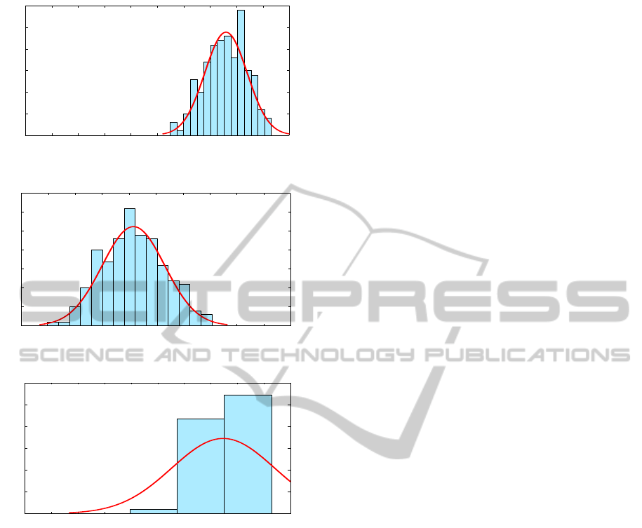
The distribution of y

cal

for the simulation time of

20 second are plotted in Figures 12 ,13 and 14. In ﬁg-

ures 12 and 14, the distribution of y

cal

measured by

and y

mod

respectively is plotted in which mean

Cycle-to-CycleTransientModelof4-strokeCombustionEngines

749

0.95 1 1.05 1.1 1.15 1.2 1.25 1.3 1.35 1.4

x 10

−4

y(k) [M

]

Probability

Figure 12: Probability distribution of y

cal

(k) using M

0.9 0.95 1 1.05 1.1 1.15 1.2 1.25 1.3 1.35 1.4

x 10

−4

y(k)[M

]

Probability

Figure 13: Probability distribution of y

cal

(k) using M

0.95 1 1.05 1.1 1.15 1.2 1.25 1.3 1.35 1.4

x 10

−4

100

120

y(k)[model]

Probability

Figure 14: Probability distribution of y

mod

(k) using model.

value of data distribution seems to be equal. That

shows the model and experimental results are seems

to be satisfactory. In ﬁgures 12 and 13, the distribu-

tion of y

cal

measured by M

and y

mod

are observed to

be different mean value.

5 CONCLUSIONS

A discrete-time model is developed and validated

with the static and transient mode. The model is also

validated using the real engine experimental data. The

y(k) calculated using the two methods of total charge

estimation and y (k) from model are compared. The

error in y(k) in case of M

(k) is higher than the cal-

culated by M

(k) due to the propagation of error in

different measured variables. In further continuing of

this research work, validation of model will be done

based on the y(k) measured using M

by the adding

of some correction factor to minimized the error at

different operating condition of engine data. A ob-

server will be established to control the air-fuel ratio,

torque and RGF using above model on cycle basis.

ACKNOWLEDGEMENTS

The authors wish to acknowledge the Toyota Motors

Corporation for the supporting in this research and

helpful discussions and Mr. Mingxin Kang for the

helping in conduct the experiment:

REFERENCES

Rizzoni G. (1999). A stochastic model for the indicated

pressure process and the dynamics of internal com-

bustion engine. IEEE Trans. Veh. Technol., vol.38, no.

3, pp.180-192, Aug. 1989.

Peyton Jones, J. C., Roberts J. B., and Landsborough K.J.

(2010). A cumulative-summation-based stochastic

knock controller. Proc. Inst. Mech. Eng., vol.224, no.

7, pp. 969-983, 2010.

Clerk, D. (1886). The gas engine. 1st ed., Longmans, Green

and Co., 1886.

Daw, C. S., Finney, C. E. A., Green, J. B., Kennel, M. B.,

and Thomas, J. F. (1996). A simple model for cyclic

variations in a spark-ignition engine. SAE Warrendale,

PA,.962086, May 1996.

Daw, C. S., Finney, C. E. A., Kennel, M. B., and Connolly,

F. T. (1998). Observing and modeling nonlinear dy-

namics in an internal combustion engine. Phys. Rev.

E., vol.57, no.3, pp. 2811-2819, 1998.

Arsie, I., Rocco, D., L., Pianese, C., and Cesare, M., D.

(2013). Estimation of in-cylinder mass and AFR by

cylinder pressure measurement in automotive Diesel

engines. IFAC World Congress, 2013.

Desantes, J. M., Galindo, J., Guardiola, C., and Dolz, V.

(2010). Air mass ﬂow estimation in turbocharged

diesel engines from in-cylinder pressure measure-

ment. Experimental Thermal and Fluid Science, vol.

34, pp. 37-47, 2010.

Yang, J., Shen, T., and Jiao, X. (2010). Model-based

stochastic optimal air-fuel ratio control with Residual

gas fraction of spark ignition engine IEEE, 2013.

Jonathan, B. V., Brian, C. K., Jagannathan, S., and

Drallmeier, J.,M (2008). Optput feedback controller

for operation of spark ignition engines at lean con-

ditions using neural networks. IEEE, vol. 16, no. 2,

March 2008.

SIMULTECH2014-4thInternationalConferenceonSimulationandModelingMethodologies,Technologiesand

Applications

750