Rapidly Exploring Random Trees-based Initialization of MPC Technique

Designed for Formations of MAVs

Zden

ek Kasl, Martin Saska and Libor P

reu

cil

Department of Cybernetics, Czech Technical University, Technick

a 2, 166 27 Prague, Czech Republic

Keywords:

Trajectory Planning, Model Predictive Control, Micro Aerial Vehicles, Rapidly Exploring Random Trees.

Abstract:

Motion planning techniques suited for initialization of Model Predictive Control based methodology applied

for complex maneuvering and stabilization of formations of Micro Aerial Vehicles are proposed in this paper.

Two approaches to initialization of the formation driving method will be described, experimentally veriﬁed,

evaluated and compared. The ﬁrst proposed method is based on multiobjective optimization of the trajectory

guess obtained by a Rapidly Exploring Random Trees technique. It represents an easy to implement and robust

method suited for off-line initialization of the formation driving algorithm. The second proposed method is

based on sequential processing of parts of the obtained trajectory. This method is well scalable and thus

applicable in large workspaces with complex obstacles. In addition, the second method enables a signiﬁcant

reduction of computational time as is shown by comparison of series of simulations in different environments.

1 INTRODUCTION

The group cooperation of autonomous robots became

an intensively studied topic in the past years. Most

recently, the research got focused on unmanned Mi-

cro Aerial Vehicles (MAVs), quadrotors, and their co-

operation. Control mechanisms and computational

power onboard of small-size MAVs enable their de-

ployment in teams with close mutual interaction.

The precisely stabilized MAV formations of compact

shapes are especially appealing for cooperative ma-

nipulation (Mellinger et al., 2013) carrying of objects

too heavy for single MAV (Maza et al., 2010) or co-

operative surveillance (Merino et al., 2007).

In this paper, we focus on a formation driving

mechanism suited for most of these applications.

The Model Predictive Control (MPC) based method

is ready to use in environments without precise exter-

nal localization system and in situations where relia-

bility and precision of global navigation satellite sys-

tems is insufﬁcient. Our developed formation driv-

ing system (Saska et al., 2014) relies on precise rel-

ative localization of neighbouring MAVs using on-

board image processing system with simple monoc-

ular cameras (Krajn

ık et al., 2014). The proposed pa-

per brings a crucial contribution to the formation driv-

ing system, which enables its deployment in complex

large workspaces due to an appropriate initial guess

of the trajectory of the formation.

In most of the path tracking and formation sta-

bilization approaches, e.g. see (Abdessameud and

Tayebi, 2011; Chen et al., 2010) and references ref-

erences cited therein, it is supposed that the desired

trajectory followed by the formation is given as an in-

put of these methods. Our method goes beyond these

works, as it does not rely on following a given trajec-

tory and the global trajectory planning is directly inte-

grated into the formation control mechanism. There-

fore, the method can continuously respond to changes

in the MAVs vicinity, while keeping the cohesion of

the immediate control inputs with the directions of

movement of the formation in the future.

In addition, the proposed novel initialization of

this MPC concept enables to extend applicability of

the method into arbitrarily complex environments and

it signiﬁcantly increases its robustness. The MPC

method relies on optimisation process that can be time

consuming if improperly initialized. In order to en-

able the trajectory optimization on-board, the opti-

mization process should be initialized with a feasible

initial trajectory.

The motion planning methods presented in this

paper are primarily suited for planning of the ini-

tial trajectory for MAV formations, but may be ef-

ﬁciently used also for planning of smooth trajecto-

ries of individual quadrotors, since MAV motion con-

straints are satisﬁed in the proposed algorithms. Both

of the proposed methods are based on the Rapidly

436

Kasl Z., Saska M. and P

reu

cil L..

Rapidly Exploring Random Trees-based Initialization of MPC Technique Designed for Formations of MAVs.

DOI: 10.5220/0005058504360443

In Proceedings of the 11th International Conference on Informatics in Control, Automation and Robotics (ICINCO-2014), pages 436-443

ISBN: 978-989-758-040-6

 2014 SCITEPRESS (Science and Technology Publications, Lda.)

exploring Random Trees (RRT) technique (LaValle,

1998). The RRT algorithm has been chosen for the

required motion planning due to its computational ef-

ﬁciency and possibility to integrate the motion con-

straints of MAVs as well as motion constraints of for-

mations of MAVs, which depend on possibly chang-

ing shape of the group. In addition, RRT provides

the output trajectory as a vector of control inputs.

Therefore, it can be directly employed as the initial-

ization of the MPC optimization process. In the pro-

posed methods, the optimality (mainly smoothness

and length) of the trajectory found by the RRT algo-

rithm is improved by consequent multiobjective op-

timization. This allows us to deﬁne the objectives,

which are similar to those used in the MPC forma-

tion driving method, already within the initialization.

The proposed approach to initialization of the MPC is

necessary for real deployment of the MAVs, where

the on-board available computational power is lim-

ited.

2 METHODS OVERVIEW

The methods proposed in this article are devised for

suitable initialization of the MPC-based approach de-

signed for guidance of formations of MAVs (Saska

et al., 2014), which is described in the ﬁrst subsec-

tion 2.1. In subsection 2.2, the RRT algorithm is de-

scribed. The RRT is used for ﬁnding an initial guess

of the input trajectory, which is further optimized be-

fore using as the initialization vector for the MPC.

2.1 Model Predictive Control

Model Predictive Control is a control algorithm orig-

inally designed for industrial applications (Mayne

et al., 2000). The method became widely used in

robotic applications with increasing computational

power of available computers.

The MPC method relies on the mathematical

model of the controlled system. The control problem,

in this case integrated formation control and trajec-

tory planning, is coded as a vector of control inputs.

Employing MPC, a solution of the control problem is

found by optimization of the vector of control inputs,

which is evaluated based on the system response pre-

diction.

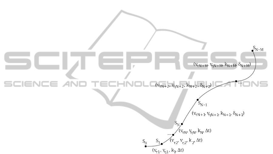
The optimization vector consists of N control in-

puts, each with constant duration ∆t, in original MPC

methods. It is forming so called prediction hori-

zon. We proposed an extension of the standard MPC

method for purposes of the trajectory planning in

(Saska et al., 2013). In the approach, the planning

horizon is extended by additional M control inputs

in order to be able to code the entire trajectory from

starting to goal state. Those M inputs have variable

time duration δ

, i = N + 1. . . N + M. Therefore, it is

possible to code long trajectories with small number

of control inputs. This setup enables the MPC to opti-

mize the entire trajectory, using the optimization vec-

tor in a form (u

, . . . , u

, u

N+1

, . . . , u

N+M

), shown in

Fig. 1. In the optimization vector, u

= (v

τi

, v

νi

, k

, t

)

is the i-th control input, v

τi

and v

νi

denote horizontal

and vertical velocity of the MAV, k

represents the cur-

vature of the given trajectory segment and t

∈

{

∆t, δ

}

is the duration of the segment.

More detailed description of the trajectory plan-

ning for formations of MAVs under MPC scheme can

be found in (Saska et al., 2014).

Figure 1: Trajectory represented as the optimization vector.

Each control input u

= (v

τi

, v

νi

, k

, t

), i = 1, . . . , N + M,

drives the MAV between consecutive states S

i−1

and S

2.2 Rapidly Exploring Random Trees

Rapidly Exploring Random Tree is a motion plan-

ning algorithm designed for search in high dimen-

sional spaces by ﬁlling them with a tree. The space–

ﬁlling tree is rooted in the starting state S

and it is

constructed in an iterative manner. The tree construc-

tion is terminated if |S

new

−S

goal

| < ε or if the number

of iterations exceeds the predeﬁned limit. The con-

stant ε is user–deﬁned precision of the planning. It

is convenient to deﬁne maximal number of iterations,

which will terminate the search in case that the de-

sired precision cannot be reached, e.g. when ε is too

small. Finally, the trajectory can be constructed from

parental references, starting from state S

N+M

which is

closest to the goal state. The detailed description of

the algorithm can be found in (LaValle, 1998).

The main advantage of this algorithm lays in its

RapidlyExploringRandomTrees-basedInitializationofMPCTechniqueDesignedforFormationsofMAVs

437

ability to accommodate kinematic and obstacle feasi-

bility constraints to the planning process. Thus guar-

anteeing the feasibility of all the trajectories contained

in the tree, e.g. when employed for nonholonomic or

kinodynamic motion planning. Moreover, the cov-

erage of the free space C

f ree

can be performed in

a short time even for environments with complex ob-

stacles. Since the control inputs u are added along

with the newly generated states, the outcome of RRT

planning is a trajectory, which is already coded as

an MPC optimization vector. However, it is not possi-

ble to guarantee optimality of the resulting trajectory,

due to randomized approach to the tree construction.

3 INITIALIZATION METHODS

The core of the designed MPC method is the opti-

mization process, which needs to be initialized with

a guess of the trajectory before the ﬁrst MPC step.

The initial guess should be a feasible trajectory in

order to assure that the method will ﬁnd a solution

which is also feasible. The RRT algorithm satisﬁes

the conditions for the MPC initialization. However

the resulting trajectories are not optimal and often

composed of many control inputs, which would sig-

niﬁcantly slow down the trajectory planning process

under the MPC scheme. The initialization methods

proposed in this article take over the advantages of

the RRT algorithm and produce suitable initial trajec-

tories for the devised trajectory planning method.

Having the raw trajectory estimate as a vector of

control inputs from the RRT algorithm (see Fig. 1),

its optimality can be improved by optimization. Sub-

sequently, it is possible to reduce the number of con-

trol inputs by merging consequent control inputs with

similar values.

3.1 Trajectory Optimization

The optimization of the initial trajectory, which re-

sults in reduction of the amount of control inputs, re-

lies on properly designed objective function. It evalu-

ates the quality of the trajectory by user-deﬁned crite-

ria in the optimization process. In order to assure that

the trajectory found by RRT algorithm is feasible for

the formation guidance, several constraints have to be

deﬁned. Both, objective and constraint functions are

described in the following sub-subsections.

3.1.1 Objective Function

In the proposed objective function, each objective is

evaluated and the ﬁnal value of the objective function

is denoted as a weighted sum of costs of the individual

objectives as

F =

∑

i=1

· F

. (1)

The weights w

are set by the user according to the im-

portance of the respective objectives. In this case,

the objectives that have to be minimized are:

Trajectory length function penalizes the length of

the trajectory as

N+M

∑

i=1

τi

+ v

νi

, (2)

where v

τi

and v

νi

are constant velocities in the i-th

control input of length t

Obstacle proximity function penalizes the trajecto-

ries that approach to obstacles closer than the safety

radius r

. The obstacle proximity function is deter-

mined as

N+M

∑

i=1



min



− r



, (3)

where d

is minimal distance from all obstacles over

the i-th interval of the trajectory and r

is critical ra-

dius. The value of the proximity function grows to

inﬁnity for d

→ r

. The trajectory is considered in-

feasible if it approaches to any of the obstacles closer

than r

Input curvature penalty is employed with the aim

to prefer straight trajectories. This function is deﬁned

N+M

∑

i=1

. (4)

Consecutive Input Difference is the key aspect

for achieving the simpliﬁcation of the trajectory for

the initialization. The aim of this function is to ob-

tain trajectories having the consecutive control input

interval values as similar as possible. Thus they can

be merged together, making the trajectory more suit-

able for the initialization of the MPC method. This

function is deﬁned for each of the control inputs as

follows:

N+M

∑

i=1

τi

− ¯v

)

, (5)

N+M

∑

i=1

νi

− ¯v

)

, (6)

N+M

∑

i=1



−



, (7)

ICINCO2014-11thInternationalConferenceonInformaticsinControl,AutomationandRobotics

438

where ¯· denotes the mean value of the individual val-

ues over all N + M control inputs.

3.1.2 Constraint Functions

The above described ﬁtness function ensures optimal-

ity of the resulting trajectory, but the feasibility of

the trajectory is not guaranteed. Therefore, it is re-

quired to apply the following set of constraints:

Motion constraints are applied to each of the con-

trol inputs u

in order to keep them in a feasible inter-

val. The bounds u

min

and u

max

are given by the con-

trolled vehicle. The control inputs are limited as

j,min

< u

j,i

< u

j,max

, i = 1 . . . N + M, (8)

where j = 1 . . . 4 denotes the individual control input

, v

, k, t) being evaluated and its respective limits.

Minimal obstacle distance ensures that the trajec-

tory will not lead to a collision with obstacles. It

also guarantees that the denominator in (3) is always

greater than zero. The constraint is deﬁned as

− d

< 0, i = 1. . . N + M, (9)

where r

is the minimal allowed distance to obstacles

and d

is the minimal distance to all obstacles of the i-

th part of the trajectory.

Final position constraint assures that the goal re-

gion is reached if the trajectory is followed. The goal

region is deﬁned by its central point X

and radius r

− X

N+M

| < r

. (10)

Vector X

N+M

denotes the last point of the followed

trajectory.

If the sequential trajectory processing is employed

(see sec. 3.4), an additional constraint

|γ

− γ| < ε

(11)

has to be considered. In the constraint, γ is the yaw

Euler angle, γ

is the desired yaw Euler angle and ε

the user–deﬁned tolerance of the ﬁnal angle.

3.2 Trajectory Simpliﬁcation

The deﬁnition of the consecutive input difference ob-

jective function ensures that the consecutive control

inputs deﬁning the trajectory will be as similar as pos-

sible after the optimization. Subsequently, the simi-

lar successive control inputs are merged into one with

adjusted parameters and prolonged time duration. It

leads to shortening the length of the optimization vec-

tor and reducing the time needed for optimization

of the trajectory. Such an initial trajectory will im-

prove the time needed for ﬁnding the optimal solution

by the MPC method, which is the main purpose of

the proposed methods.

Having two consecutive control inputs u

τ1

, v

ν1

, k

, t

) and u

= (v

τ2

, v

ν2

, k

, t

), it is pos-

sible to merge them into one input, if they fulﬁl three

conditions. The ﬁrst two conditions concern the ve-

locities of the consecutive control inputs:

τ1

− v

τ2

| < ε

vτ

(12)

and

ν1

− v

ν2

| < ε

vν

, (13)

where ε

vτ

and ε

vν

denote the user-deﬁned velocity

tolerance. This tolerance has to be deﬁned with re-

spect to the difference of the ﬁnal state, which may

be caused by merging of the two consecutive con-

trol intervals. The difference is proportional to the re-

spective tolerance and to the duration of the interval.

In this case, the difference in horizontal or vertical

movement may be compensated by shortening or pro-

longing the duration of the interval and by appropri-

ate adjusting the average velocity values. However,

an extra attention has to be paid to respecting the lim-

its u

min

and u

max

The third condition is deﬁned as

− k

| < ε

. (14)

The analysis of inﬂuence of curvature difference be-

tween two consecutive segments to the ﬁnal state after

their merging is not as straightforward as in the pre-

ceding case. The worst case scenario is depicted in

Fig. 2. Applying the control input u

moves the MAV

to γ = 180

◦

along a circular trajectory and applying

the control input u

moves it by another 180

◦

along

a circular trajectory with different curvature. The po-

sition error is then equal to double of the difference

∆r =

− k

. (15)

In this case, the tolerance should be determined

with respect to the biggest allowed curvature. It is

shorter trajectory to travel 180

◦

around a circular tra-

jectory with maximal curvature and therefore it is

more likely that the worst case scenario will occur.

With decreasing curvature, the crossing point moves

towards 90

◦

(see Fig. 3) and 45

◦

(see Fig. 4) and

the resulting difference becomes smaller than the dou-

ble of radius difference.

With all merging criteria deﬁned, it is possible

to loop through the trajectory and merge together

the consecutive control intervals that fulﬁl the con-

ditions of similarity. The control inputs applied on

RapidlyExploringRandomTrees-basedInitializationofMPCTechniqueDesignedforFormationsofMAVs

439

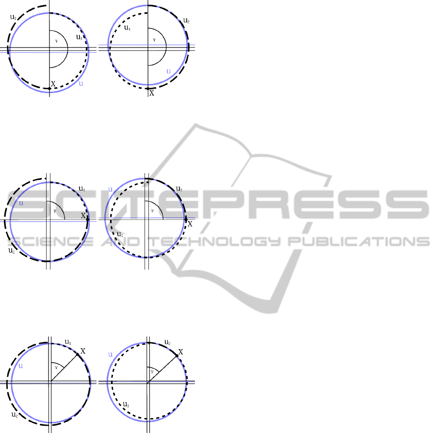
(a) u

to u

transition (b) u

to u

transition

Figure 2: The worst case scenario occurs when merging

two circular trajectories that cross at γ = 180

◦

. The dif-

ference in the ﬁnal state is equal to the radius difference

∆r. The lighter color denotes the average control input u,

replacing control inputs u

and u

(a) u

to u

transition (b) u

to u

transition

Figure 3: Crossing at γ = 90

◦

. The difference in the ﬁnal

state is smaller than the radius difference ∆r. The lighter

color denotes the average control input u, replacing control

inputs u

and u

(a) u

to u

transition (b) u

to u

transition

Figure 4: Crossing at γ = 45

◦

and less, which is the scenario

most likely to occur for control inputs with small curvatures.

The difference in the ﬁnal state is also smaller than the ra-

dius difference ∆r. The lighter color denotes the average

control input u, replacing control inputs u

and u

the merged consecutive intervals are obtained as fol-

lows:

u =



¯v

, ¯v

k, t



, (16)

where the operation ¯· denotes the average value of

the two inputs u

and u

3.3 Naive Approach

This approach to a suitable initialization of the MPC

method is an intuitive employment of the de-

scribed optimization approach and the proposed tra-

jectory simpliﬁcation method to a trajectory found by

the RRT algorithm. The main idea is that the whole

trajectory obtained from the RRT algorithm is simpli-

ﬁed together, using the previously described methods.

The trajectory found by the RRT algorithm is

composed of many control inputs and it is usually far

from the optimal result. The approach to construc-

tion of the space-ﬁlling tree suggests that the trajec-

tory will often change direction and thus it is difﬁ-

cult to simplify. This is the reason why the trajec-

tory found by the RRT is pre-optimized, using the ap-

proach described in section 3.1. The objective func-

tion of the optimization process was designed with

the aim of uniﬁcation of the consecutive intervals of

the trajectory. Therefore, it is possible to employ

the trajectory simpliﬁcation method described in sec-

tion 3.2 and merge all control inputs with similar val-

ues together. In a general case, the simpliﬁed trajec-

tory is optimal with respect to the objective function

deﬁned in section 3.1 and it is described by less con-

trol inputs. Thus it is suitable for the initialization of

the MPC.

The main weakness of this approach is that it suf-

fers form the length of the optimization vector gener-

ated by the RRT algorithm. In some cases, the opti-

mization may take minutes to complete. This is why

the naive approach is suitable merely for applications

that allow ofﬂine pre-calculation of the initial trajec-

tory with no time constraints.

3.4 Sequential Processing

The sequential processing approach exploits the fact

that the time consumed by the optimization grows as

O(n

), where n is the number of control inputs de-

scribing the trajectory, i.e. n = |u| · (N + M). There-

fore, piecewise processing of the trajectory speeds up

the optimization process.

In order to preserve start and end state of

the whole trajectory, start and end states of each of

the processed parts of the trajectory should be ﬁxed.

Moreover, the yaw Euler angle γ in each start and

end conﬁguration has to be ﬁxed as well, in order to

enable putting the trajectory smoothly back together.

The optimization of the pieces of the trajectory is im-

plemented according to section 3.1 and the conse-

quent simpliﬁcation is performed as described in sec-

tion 3.2.

Once the simpliﬁcation of smaller pieces of

ICINCO2014-11thInternationalConferenceonInformaticsinControl,AutomationandRobotics

440

the trajectory is complete, the overall optimization has

to be performed in order to improve the trajectory to

its ﬁnal state. Subsequently, the simpliﬁcation is done

producing the ﬁnal trajectory.

In some cases, the piecewise reduction of the tra-

jectory does not affect the result and the number of

control inputs remains the same. Then, it is efﬁ-

cient to replan the RRT trajectory estimate. The prob-

ability of occurrence of this problem can be re-

duced by planning several trajectories, exploiting

the time efﬁciency of the RRT algorithm in compari-

son with the time demanding trajectory optimization

in the post-processing phase. From the obtained set,

the best candidate trajectory can be selected e.g. by

evaluating with subset of objectives deﬁned in opti-

mization objective function in section 3.1.

If a multi-core processor is available, it is possible

to run this method as a parallel processing. Running

the optimization of the parts of the trajectory in paral-

lel threads fully exploit the beneﬁts of the processor.

4 EXPERIMENTS

The experimental veriﬁcation of the properties of

the proposed methods is described in this sec-

tion. The RRT algorithm uses kinematic model

described in (Saska et al., 2014) employing con-

straints shown in tab. 1. Each state S

new

is se-

lected from a set of candidate states that are gener-

ated by applying a set of control inputs U. The set

U contains combinations of control inputs with

horizontal velocity v

= 0.6 m · s

−1

, normal veloci-

ties v

∈

{

−0.3, 0.0, 0.3

}

m · s

−1

and curvatures k ∈

{

−1.0, 0.0, 1.0

}

−1

. The duration of the control

inputs is reduced with increasing number of itera-

tions, as t = 2.5 s for 1 < i < 2000; t = 0.5 s for

2001 < i < 5000 and t = 0.1 s for 5001 < i < 10000.

The decreasing length of control inputs helps to main-

tain rapid coverage of the free space and to reduce

size of the tree. Moreover, the decreasing length of

the control inputs helps to ﬁnd trajectories that are

composed of fewer–longer control inputs, rather than

more shorter control inputs. A counterexample with

ﬁxed control input duration t = 0.1 s is also presented.

Maximal number of iterations of the RRT algorithm is

set to m

iter

= 10000.

The choice of the duration of the control input in-

ﬂuences the level of detail of planning. Therefore, it is

crucial to pay attention to its choice if the algorithm

is used for planning in an environment with narrow

passages with respect to the formation size.

The trajectory merging constants were set accord-

ing to section 3.2 as follows: ε

vτ

= 0.01 m · s

−1

; ε

vν

Table 1: Kinematic constraints of an MAV.



m · s

−1





m · s

−1





−1



t [s]

min

0 −0.3 −1 0

max

0.6 0.3 1 10

0.01m · s

−1

and ε

= 0.01m

−1

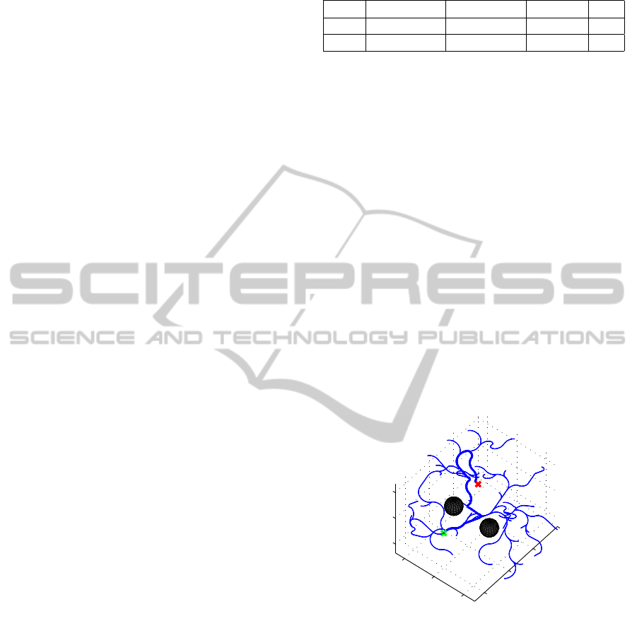
4.1 Tree and Trajectory

An example of the space-ﬁlling tree generated by

the RRT algorithm is shown in Fig. 5. The bold line

denotes the resulting trajectory found by the algo-

rithm.

As you may notice, the trajectory does not end in

the desired goal point exactly, which is ﬁne for pur-

poses of testing. In real deployment, if the distance

between the ﬁnal point of the trajectory and the de-

sired goal point is higher than a predeﬁned threshold,

the trajectory has to be replanned.

The time efﬁciency of the RRT algorithm can be

exploited by planning several trajectories and taking

the most suitable one for the optimization. For ex-

ample, a number of control inputs, ﬁnal distance to

goal point, existence of a loop within the trajectory or

length of the trajectory can be taken as a criterion.

−5

x[m]

y[m]

z[m]

Figure 5: Space-ﬁlling tree, with resulting trajectory (bold).

4.2 Trajectory Optimization

The comparison of the raw trajectory obtained from

the RRT algorithm and the optimization result is

shown in Fig. 6. The initial trajectory (dark) was

coded using 16 control inputs. The number of con-

trol inputs was reduced to 10 (light).

It may happen that the trajectory found by

the RRT algorithm contains a loop. This situation is

depicted in the horizontal plane projection in Fig. 7.

Again, the dark trajectory is the raw trajectory ob-

tained from the RRT algorithm and the light one is

RapidlyExploringRandomTrees-basedInitializationofMPCTechniqueDesignedforFormationsofMAVs

441

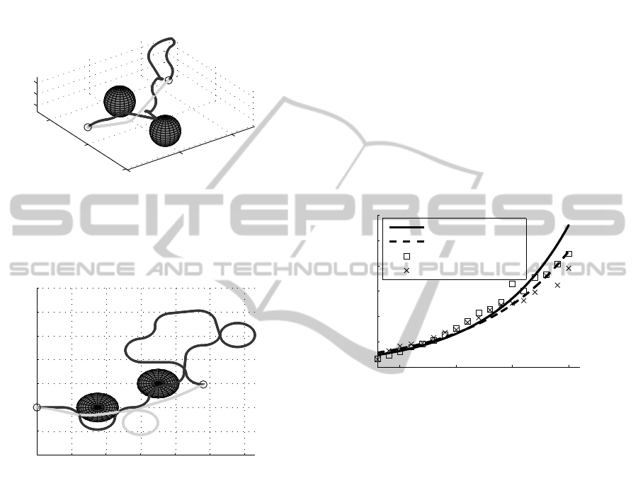
the result of the optimization process. The control in-

put reduction is not so signiﬁcant as in the previous

case due to the occurrence of the loop. Here, 25 orig-

inal control inputs were reduced to 22. Therefore, it

is important to detect and reject loopy trajectories.

−5

−1

x[m]

y[m]

z[m]

Figure 6: Comparison of trajectory generated by the RRT

algorithm (dark) with trajectory after optimization (light).

The circles denote start and end points of both trajectories.

0 2 4 6 8 10 12

−4

−2

x[m]

y[m]

Figure 7: Example of trajectory containing loop before op-

timization (dark) and after optimization (light). The black

circles denote start and end points of the trajectory.

4.3 Optimization Methods Comparison

The presented methods are compared concerning

the time consumption in this sub-section. The ﬁrst

two experiments were performed in obstacle-free en-

vironment and in an environment with obstacles.

The third experiment shows properties of presented

algorithms when treating long trajectories (over 100

control inputs). This last scenario may happen if a de-

tailed space coverage by the RRT algorithm is re-

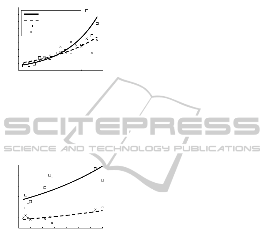
quired, e.g. in a narrow passage. In all of the ﬁg-

ures presented in this subsection, the measured data

(rectangular and cross marks) were interpolated with

an exponential function in order to illustrate the rate

of time consumption increase.

4.3.1 Obstacle–free Environment

In this experiment, each of the proposed methods

was run 1000 times with ﬁxed start conﬁguration and

varying goal. All the time measurements were col-

lected and the graph of average time consumption is

shown in Fig. 8. The time consumption t is shown

with respect to the number of control inputs n describ-

ing the trajectory. The length of the trajectory part for

sequential processing was set to 4 control inputs.

The graph shows that the average time con-

sumption in the obstacle-free environment is simi-

lar. The sequential method time consumption is inﬂu-

enced by the choice of number of control inputs for

sub-optimization. The graph shows, that the sequen-

tial method ﬁnds solution faster than the naive method

for trajectories with more control inputs.

10 15 20 25

x 10

n [−]

t [ms]

Naive method

Sequential method

Naive−data

Sequential−data

Figure 8: Comparison of performance of the proposed

methods in obstacle-free environment. The variable n de-

notes the number of control inputs describing the trajectory.

4.3.2 Environment with Obstacles

The sequential processing method was used with

the same setup as in the preceding experiment. An en-

vironment with 52 spherical obstacles was used for

veriﬁcation of the algorithm performance. Both meth-

ods were run 100 times and the time measurements

were collected. The comparison in Fig. 9 shows

that the maximal time consumption of the sequen-

tial method is signiﬁcantly smaller in comparison to

the naive method.

4.3.3 Fixed RRT Control Input Duration

In case that a more detailed coverage of the free

space is required, the tree will produce much longer

trajectory than in the preceding two scenarios, i.e.

the trajectory is composed of over 100 control in-

puts. Both methods were run 100 times in this experi-

ment in an environment with four spherical obstacles.

The length of sub-optimization part of trajectory was

ICINCO2014-11thInternationalConferenceonInformaticsinControl,AutomationandRobotics

442

10 15 20

x 10

n [−]

t [ms]

Naive method

Sequential method

Naive−data

Sequential−data

Figure 9: Comparison of performance of the proposed

methods in environment with obstacles. The variable n de-

notes the number of control inputs describing the trajectory.

set to 10 control inputs. The comparison of average

time consumption is shown in Fig. 10.

The graph shows that the time consumption of

the naive method rapidly grows with increasing num-

ber of control inputs. The increase of time consump-

tion of the sequential method is more gradual due to

the reduction of the number of control inputs.

165 170 175 180 185 190 195 200

x 10

n [−]

t [ms]

Figure 10: Comparison of performance of the proposed

methods when planning long trajectories. The legend re-

mains the same as in previous ﬁgures. The variable n de-

notes the number of control inputs describing the trajectory.

5 CONCLUSIONS

The motion planning methods presented in this paper

respect kinematic constraints of the particular MAVs

as well as the entire MAV formation. The resulting

trajectory is coded as a vector of control inputs, i.e.

in the form required by the MPC method. There-

fore, these methods are suitable for initial trajectory

planning for formations of MAVs. The proposed ap-

proaches increase the time efﬁciency of the method.

When employing the methods in a complex en-

vironment, an attention has to be paid to the choice

of the merging constants as well as to the setup of

the RRT algorithm. The experimental veriﬁcation

showed that the sequential processing method is more

efﬁcient, compared to the naive method. If the tra-

jectory guess for the method is selected from a set

of trajectories computed using the RRT algorithm,

the time required to ﬁnd a solution can be signiﬁcantly

reduced.

ACKNOWLEDGEMENTS

This work was supported by internal CTU grant no.

SGS14/073/OHK3/1T/13, GA

CR postdoc grant no.

P103-12/P756 and M

SMT grant under Kontakt II no.

LH11053.

REFERENCES

Abdessameud, A. and Tayebi, A. (2011). Formation control

of vtol unmanned aerial vehicles with communication

delays. Automatica, 47(11):2383 – 2394.

Chen, J., Sun, D., Yang, J., and Chen, H. (2010).

Leader-follower formation control of multiple non-

holonomic mobile robots incorporating a receding-

horizon scheme. Int. Journal Robotic Research,

29:727–747.

Krajn

ık, T., Nitsche, M., Faigl, J., Van

ek, P., Martin, S.,

reu

cil, L., Duckett, T., and Mejail, M. (2014). A

practical multirobot localization system. Journal of

Intelligent and Robotic Systems, pages 1–24.

LaValle, S. M. (1998). Rapidly-exploring random trees a

new tool for path planning.

Mayne, D. Q., Rawlings, J. B., Rao, C. V., and Scokaert,

P. O. (2000). Constrained model predictive control:

Stability and optimality. Automatica, 36(6):789–814.

Maza, I., Kondak, K., Bernard, M., and Ollero, A. (2010).

Multi-uav cooperation and control for load transporta-

tion and deployment. Journal of Intelligent and

Robotic Systems, 57(1-4):417–449.

Mellinger, D., Shomin, M., Michael, N., and Kumar, V.

(2013). Cooperative grasping and transport using mul-

tiple quadrotors. In Distributed autonomous robotic

systems, pages 545–558. Springer.

Merino, L., Caballero, F., Ferruz, J., Wiklund, J., Forss

en,

P.-E., and Ollero, A. (2007). Multi-uav cooperative

perception techniques. In Multiple Heterogeneous

Unmanned Aerial Vehicles, pages 67–110. Springer.

Saska, M., Kasl, Z., and P

reu

cil, L. (2014). Motion plan-

ning and control of formations of micro unmanned

aerial vehicles. In 19th World Congress of IFAC. To

be published.

Saska, M., Mej

ıa, J., Stipanovi

c, D. M., Von

asek, V.,

Schilling, K., and P

reu

cil, L. (2013). Control and

navigation in manoeuvres of formations of unmanned

mobile vehicles. European Journal of Control,

19(2):157–171.

RapidlyExploringRandomTrees-basedInitializationofMPCTechniqueDesignedforFormationsofMAVs

443