Nonlinear Feedback Control and Artiﬁcial Intelligence Computational

Methods applied to a Dissipative Dynamic Contact Problem

Daniela Danciu

, Andaluzia Cristina Matei

, Sorin Micu

2,3

and Ionel Rovent¸a

Department of Automation, Electronics and Mechatronics, University of Craiova, 200585, Craiova, Romania

Department of Mathematics, University of Craiova, 200585, Craiova, Romania

Institute of Mathematical Statistics and Applied Mathematics, 70700, Bucharest, Romania

Keywords:

Hyperbolic partial differential equation, Contact problem, Method of Lines, Galerkin method, Cellular Neural

Networks, Computational methods, Neuromathematics.

Abstract:

In this paper we consider a vibrational percussion system described by a one-dimensional hyperbolic partial

differential equation with boundary dissipation at one extremity and a normal compliance contact condition at

the other extremity. Firstly, we obtain the mathematical model using the Calculus of variations and we prove

the existence of weak solutions. Secondly, we focus on the numerical approximation of solutions by using a

neuromathematics approach – a well-structured numerical technique which combines a speciﬁc approach of

Method of Lines with the paradigm of Cellular Neural Networks. Our technique ensures from the beginning

the requirements for convergence and stability preservation of the initial problem and, exploiting the local con-

nectivity of the approximating system, leads to a low computational effort. A comprehensive set of numerical

simulations, considering both contact and non-contact cases, ends the contribution.

1 INTRODUCTION

The purpose of the paper is twofold. Firstly, we

verify, on a new mathematical model from Con-

tact Mechanics, a well-structured technique for solv-

ing hyperbolic partial differential equations (hPDEs),

by using Method of Lines (MoL) combined with

the features and ﬂexibility of Cellular Neural Net-

works (CNNs) – nonlinear processing devices having

a large amount of applications from image processing

to numerical solving of differential equations. This

is a neuromathematics approach, i.e., according to

(Galushkin, 2010), an approach used for solving both

non-formalized (or weakly formalized) and formal-

ized problems using the neural networks paradigm.

Our approach addresses the formalized-type prob-

lems where the structure of the neural network is

based only on the “natural parallelism” of the problem

itself and does not need a learning process based on

experimental data. We have already successfully ap-

plied our technique for the overhead crane with non-

homogeneous cable (Danciu, 2013a), the torsional

stick slip oscillations in oilwell drillstrings (Danciu,

2013b) and the controlled ﬂexible arm of an ocean

vessel riser (Danciu and R˘asvan, 2014).

It is assumed that our method is even more effec-

tive for high dimensions, where the well-organized

technique may have the following advantages: a) ac-

curacy (for example, fewer rounding errors), b) ro-

bustness to ill numerical conditioning and c) use of

existing high-performance software for solving ordi-

nary differential equations (ODEs).

Secondly, we study a particular robotic system of

type vibrational percussion system, which is mod-

elled by a one-dimensional hPDE with a dissipative

boundary condition at one extremity and a contact

nonlinear phenomenon at the other extremity. The

study concerns mathematical modelling of the sys-

tem, existence of the weak solutions for the hPDE

problem, numerical approximation and asymptotic

behavior. The problem can be viewed as a structure

with nonlinear feedback and reference signal. From

the mathematical point of view, the main difﬁculties

reside in the nonlinearity of the problem, the lack of a

regularization effect of solutions, possibly the effects

of discretization on the dissipative mechanism.

The rest of paper is organized as follows. Sec-

tion 2 deals with mathematical modelling of the sys-

tem via Calculus of variation methods. Section 3 fo-

cuses on the study of the existence of weak solutions

for the hPDE problem, whereas Section 4 is devoted

to numerical approximation of the solution. We im-

528

Danciu D., Matei A., Micu S. and Roven¸ta I..

Nonlinear Feedback Control and Artiﬁcial Intelligence Computational Methods applied to a Dissipative Dynamic Contact Problem.

DOI: 10.5220/0005055005280539

In Proceedings of the 11th International Conference on Informatics in Control, Automation and Robotics (ICINCO-2014), pages 528-539

ISBN: 978-989-758-039-0

 2014 SCITEPRESS (Science and Technology Publications, Lda.)

g(t)

f(t,x)

Figure 1: Elastic rod with boundary conditions: 1) a dash-

pot and time-varying external force at x = 0 and 2) a de-

formable obstacle with normal compliance and initial gap

at x = L.

plement the approximating system of ODEs by using

the CNN paradigm in order to exploit the regularity,

parallelism and matrix sparsity of the new problem.

The section provides a comprehensive set of numer-

ical simulations, considering both contact and non-

contact cases. Concluding remarks end the paper.

2 THE MATHEMATICAL MODEL

We consider an elastic rod with a dashpot attached to

the left end x = 0. At the opposite extremity x = L the

rod can come in contact with a deformable obstacle

with normal compliance of stiffness

, ε > 0. The ob-

stacle is located at a distance l (often called the initial

gap) to the right of the point x = L. The rod is sub-

jected to a body force of density f in the x-direction

and to an external force g(t) which acts at the extrem-

ity x = 0 as shown in Figure 1

In order to obtain the mathematical model, we use

the Calculus of variation methods. For our case, the

kinetic E

and the potential E

energies are

(t) =

ρ(x)A(x) ˙u

(t,x)dx

(t) =

A(x)σ

(t,x)dx.

(1)

Herein, u represents the longitudinal displacement;

the internal longitudinal force in the rod is given by

σ(x) = Eu

(t,x) where E > 0 represents the Young

modulus of the material; ρ is the density of the ma-

terial; A is the cross-sectional area of the rod. In (1)

and in the sequel ˙u denotes the ﬁrst time derivative

of u and u

denotes the ﬁrst derivative with respect to

space variable x. Taking into consideration the dissi-

pative forces due to viscous friction at both extrem-

ities of the rod h

(t), h

(t), the external force g(t)

and the axial force of density along the rod f(t,x),

the work W

done by these forces is

(t) = h

(t)u(t, 0) + g(t)u(t, 0) + h

(t)(u(t,L) −l)

f(t, x)u(t, x)dx.

(2)

Consider the functional associated to the Hamilton

variational principle

I(t

) =

(t) −E

(t) +W

(t))dt (3)

with arbitrary t

, t

and introduce the standard Euler-

Lagrange variations

u(t,x) = ¯u(t, x) + ςµ(t,x) (4)

where ¯u(t,x) is the basic trajectory and ςµ(t,x) is the

variation of ¯u(t,x). The condition for the functional

(3) to be minimal along the trajectories of the system

will give, after some lengthy but straightforward ma-

nipulations, the following equations

−ρ(x)A(x)

¯u+ (A(x)E ¯u

)

+ f(t,x) = 0

A(0)E ¯u

(t,0) + h

(t) + g(t) = 0

−A(L)E ¯u

(t,L) + h

(t) = 0

(5)

At x = L we shall introduce the contact condition, i.e.

the last equation in (5) will be replaced by

(t,L) = −p(u(t,L) −l), t ∈ (0, T), (6)

with function p(·), having the measure unit of stress,

described below in this section. Considering the dis-

sipative force due to the damper, at x = 0, h

(t) =

−ku

(t,0) to be in the opposite direction of motion

and, the case of a uniform rod, the equations (5) – (6)

become (with an abuse of notation u := ¯u)

ρ(x)A(x) ¨u(t, x) −EA(x)u

(t,x) = f(t,x)

A(x)Eu

(t,0) −k ˙u(t,0) = −g(t)

(t,L) = −p(u(t,L) −l)

(7)

Considering A(x) = A > 0 and ρ(x) = ρ > 0, the

mechanical model leads us to the following boundary

value problem with initial data











ρ ¨u(t,x) −E u

(t,x) =

f(t, x) x ∈ (0, L),

t ∈ (0, T)

AEu

(t,0) = k ˙u(t,0) −g(t) t ∈ (0, T)

(t,L) = −p(u(t,L) −l) t ∈ (0, T)

u(0,x) = u

(x) x ∈ (0,L)

˙u(0,x) = u

(x) x ∈ (0,L).

(8)

NonlinearFeedbackControlandArtificialIntelligenceComputationalMethodsappliedtoaDissipativeDynamicContact

Problem

529

where the contact condition is modelled with the fol-

lowing normal compliance function:

p(r) =



−1

r if r ≥ 0

0 if r < 0.

(9)

Herein, ε is the stiffness coefﬁcient. By using the nor-

mal compliance contact condition (6), the unilateral

Signorini’s condition

u(t,L) ≤ l, u

(t,L) ≤ 0, u

(t,L)(u(t,L) −l) = 0

is relaxed; formally, Signorini’s nonpenetration con-

dition is obtained in the limit ε →0. Thus, the contact

with a rigid obstacle can be viewed as a limit case of

contact with deformable support whose resistance to

compression subsequently increases.

The normal compliancecondition was proposed in

(Martins and Oden, 1987) with p(r) = c(r

)

where

c, m > 0 and r

= max{0, r}. Then it was used in

a large number of publications, see e.g. (Anders-

son, 1991; Andersson, 1995; Han and Sofonea, 2002;

Kikuchi and Oden, 1988; Klarbring and Shillor, 1988;

Klarbring and Shillor, 1991; Rochdi and Sofonea,

1998).

3 EXISTENCE OF SOLUTIONS

This section is devoted to study the existence of weak

solutions of (8) assuming that f ∈ L

((0,T) ×(0,L))

and (u

) ∈V := H

(0,L) ×L

(0,L). Without loss

of generality but simplifying the writing everywhere

in this section, we shall set E = 1, k = 1 and ρ ≡ 1.

First of all, note that, if u is a classical solution of (8),

we obtain that, for every v ∈ H

(0,L), the following

relation holds for almost any t ∈[0,T]

h¨u(t), vi+ hu

(t),v

i+ ( ˙u(t,0) + g(t))v(0)

+ p(u(t,L) −l)v(L) = hf(t),vi. (10)

In (10) and in the sequel, h , i denotes the inner prod-

uct in L

(0,L). By integrating in time (10), we obtain

that, for almost any t ∈[0,T],

h˙u(t), vi−





(s),v

ids

+ v(0)

g(s)ds+ (u(t,0) −u

(0))v(0)

+ v(L)

p(u(s,L) −l)ds =

hf(s),vids. (11)

These relations allow us to give the deﬁnition of a

weak solution of (8).

DEFINITION 3.1. A function u ∈C

([0,T];L

(0,L))∩

C([0, T];H

(0,L)) is a weak solution of (8) if it veri-

ﬁes (11) for any v ∈ H

(0,L), u(0) = u

and ˙u(0) =

Note that a solution u ∈ C

([0,T];L

(0,T)) ∩

([0,T];H

(0,L)) of (11), also veriﬁes (10) and it

is a strong (classical) solution of (8).

The main result of this section is the following.

THEOREM 3.1. Given T > 0, u

∈ H

(0,L), u

∈

(0,L), f ∈ L

((0,T) × (0,L)) and g ∈ L

(0,T),

equation (8) has a weak solution (in the sense of Def-

inition 3.1)

u ∈C

([0,T];L

(0,L)) ∩C([0, T];H

(0,L)). (12)

For the proof of Theorem 3.1 we use the well-

known Galerkin method (see, for instance, (Lions,

1969) and (Kim, 1989) where this method is applied

in similar cases). In order to do that, let (w

)

k≥1

⊂

∞

(0,L) be a basis of the space L

(0,L). For each

m ≥ 1, we deﬁne the space

= Span{w

,...,w

Let us ﬁrst prove three technical lemmas.

LEMMA 3.1. Let m ≥ 1. For any (a

)

1≤j≤m

∈ R

and (a

)

1≤j≤m

∈ R

, there exists a unique function

∈C

([0,T];V

) which veriﬁes (10) for any v ∈V

and it is of the form

(t,x) =

∑

j=1

(t)w

(x), (13)

with (a

)

1≤j≤m

⊂ C

[0,T], a

(0) = a

and

′

(0) = a

Proof. Since any function in C

([0,T];V

) is of the

form (13) the result follows if we prove that there

exists a unique sequence (a

)

1≤j≤m

⊂C

[0,T] with

(0) = a

and a

′

(0) = a

such that for each 1 ≤

i ≤ m we have that

∑

j=1

¨a

(t)





∑

j=1

(t)



j,x

(t),w

i,x



∑

j=1

˙a

(t)w

(0)w

(0) + g(t)w

(0)

+ p

∑

j=1

(t)w

(L) −l

(L) = hf(t),w

(14)

In order to simplify the writing we introduce the

following notations

A = (A

)

1≤j,i≤m

= (hw

1≤j,i≤m

∈ R

−1

= (α

)

1≤j,i≤m

Note that, due to the linear independence of the

functions (w

)

j≥1

in L

(0,L), the matrix A is invert-

ible. For 1 ≤ j, i ≤ m we also note

j,x

i,x

i = β

∈ R, w

(0)w

(0) = γ

∈ R,

ICINCO2014-11thInternationalConferenceonInformaticsinControl,AutomationandRobotics

530

Therefore, the system (14) can be rewritten as fol-

lows,



˙a

(t) = b

(t)

(t) = c

(t)

where

(t) = −

∑

i=1

∑

k=1

(t)α

−

∑

i=1

∑

k=1

(t)α

+ g(t)

∑

i=1

(0)

− p

∑

k=1

(t)w

(L) −l

∑

i=1

(L)

∑

i=1

hf(t), w

i. (15)

Notice that c = (c

,...,c

)

∗

∈ C([0, T];R

Here and in the sequel x

∗

denotes the adjoint of the

vector x.

Let y ∈ C

([0,T];R

), y = (a,b)

∗

a = (a

,...,a

)

∗

∈ C([0, T];R

b = (b

,...,b

)

∗

∈C([0,T];R

The system (14) can be rewritten now as follows.

˙y(t) = F(y)(t)

where

F :C

([0,T];R

) →C

([0,T];R

) F y = (b,c)

∗

The function F is a Lipschitz continuous one. Indeed,

if we take t ∈ [0,T] we have that

k(Fy

−Fy

)(t)k

≤ k

(kb

(t) −b

(t)k

+ kc

(t) −c

(t)k

)

≤ k

(kb

(t) −b

(t)k

∑

j=1

(t) −c

(t)|).

(16)

Since

(t) −c

(t)| ≤

∑

i,k=1

(t) −a

(t)|α

∑

i,k=1

(t) −b

(t)|α



∑

k=1

(t)w

(L) −l

−p

∑

k=1

(t)w

(L) −l



∑

i=1

(L), (17)

as p is a Lipschitz continuous function we deduce

that

(t) −c

(t)| ≤ k

(ka

(t) −a

(t)k

+ kb

(t) −b

(t)k

). (18)

By (16), (17) and (18) we can write

k(Fy

−Fy

)(t)k

≤ k

(ka

(t) −a

(t)k

+ kb

(t) −b

(t)k

)

≤ k

max

t∈[0,T]

(t) −y

(t)k

. (19)

Therefore,

kFy

−Fy

C([0,T];R

)

≤ k

−y

C([0,T];R

)

Since (14) is a system of ordinary differential

equations with a Lipschitz nonlinear term, it fol-

lows that there exists a unique solution (a

)

1≤j≤m

⊂

[0,T] with a

(0) = a

and ˙a

(0) = a

of (14).

LEMMA 3.2. The sequence (u

)

m≥1

given by

Lemma 3.1 is uniformly bounded in the space

∞

([0,T];H

(0,L)) ∩H

([0,T];L

(0,L)).

Proof. Since u

veriﬁes (10) for any v ∈V

it follows

that,

h¨u

(t),ϕ

(t)i+ hu

m,x

(t),ϕ

m,x

(t)i

+ ( ˙u

(t,0) + g(t))ϕ

(t,0)

+ p(u

(t,L) −l)ϕ

(t,L) = hf(t),ϕ

(t)i, (20)

for any ϕ

∈C

([0,T];V

). Now, if we take ϕ

= ˙u

in (20) we deduce that



˙u

(t,x)dx+

m,x

(t,x)dx

(p(u

(t,L) −l))



+( ˙u

(t,0))

+ g(t) ˙u

(t,0) = hf(t), ˙u

(t)i.

If we deﬁne the energy of the solution by

(t) =

˙u

(t,x)dx+

m,x

(t,x)dx

(p(u

(t,L) −l))

we obtain from the previous relation that

(t) ≤ hf(t), ˙u

(t)i+

(t).

Let t ∈ [0, T]. After integration between 0 and t we

get

(t) ≤ E

(0) +

˙u

(s,x)dxds

(s)ds+

(s,x)dxds

and from this we deduce

(t) ≤ E

(0) +

(s)ds

NonlinearFeedbackControlandArtificialIntelligenceComputationalMethodsappliedtoaDissipativeDynamicContact

Problem

531

(s,x)dxds+

(s)ds.

By using a Gronwall inequality we can write

(t) ≤



(0) +

(s)ds

(s,x)dxds



≤



(0) +

(s)ds

(s,x)dxds



Therefore, we have that

˙u

(t,x)dx ≤



(0) +

(s)ds

(s,x)dxds



m,x

(t,x)dx ≤



(0) +

(s)ds

(s,x)dxds



The required boundedness properties are straight-

forward consequences of the last two inequali-

ties.

LEMMA 3.3. Suppose that

∑

j=1

→ u

in H

(0,L) as m → ∞, (21)

∑

j=1

→ u

in L

(0,L) as m →∞. (22)

There exists a subsequence (u

)

k≥1

of the sequence

)

m≥1

given by Lemma 3.1 and a function u ∈

([0,T];L

(0,L)) ∩C([0, T];H

(0,L)) such that

⇀

∗

u in L

∞

([0,T];H

(0,L)) (23)

⇀ u in H

([0,T];L

(0,L)). (24)

Proof. The existence of u follows from the bounded-

ness properties from Lemma 3.2.

Now we have all the ingredients needed to prove

the main result of this section.

Proof of Theorem 3.1. Let u be the function obtained

in Lemma 3.3. We provethat u veriﬁes (11). From the

linearity and continuity of the left hand side of (11) in

v ∈ H

(0,L), it follows that (11) is equivalent to



˙u(t), w



−







(s),w

j,x



+ (u(t,0) −u

(0))w

(0) + g(t)w

(0)

+ w

(L)

p(u(s,L) −l)ds =



f(s),w



ds,

(25)

for each j ≥ 1. Now, the fact that u veriﬁes (25) fol-

lows by taking the limit when m tends to inﬁnity in

(14), by using the convergence properties (21)-(24)

and by integrating in time from 0 to t.

Finally, we remark that, from (10), the unique-

ness of a classical solution u ∈ C

([0,T];L

(0,T)) ∩

([0,T];H

(0,L)) of (8) can be easily proved. The

uniqueness of a weak solution is more difﬁcult to

show and it will be addressed in a future work.

4 NUMERICAL

APPROXIMATION OF

SOLUTIONS

As Bertrand Russell said, “although this may seem a

paradox, all exact science is dominated by the idea of

approximation”. Numerical approximations are even

more useful for problems which cannot be analyti-

cally solved. In order to numerically solve the mixed

initial boundary value problem for hPDE (8), we con-

sider an approach of Method of Lines which employs

the paradigm of Cellular Neural Networks.

The Method of Lines is a general concept rather

than a speciﬁc method and, can be used for solving

hyperbolic PDEs. The overall philosophy is to sep-

arately cope with the space and time discretization.

The ﬁrst step is to choose an adequate method for dis-

cretizing hPDE with respect to the space variables and

incorporate the boundary conditions. “The spectrum

of this discrete operator is then used as a guide to

choose an appropriate method to integrate the equa-

tions through time” (Hyman, 1979).

4.1 The Approximating System Via

Method of Lines

The main idea of our numerical technique is the fol-

lowing. For the ﬁrst step of MoL – the discretization

of derivatives with respect to the space coordinates

by taking into account the boundary conditions – we

use an approach which, according to (Halanay and

R˘asvan, 1981), ensures for the approximating system

ICINCO2014-11thInternationalConferenceonInformaticsinControl,AutomationandRobotics

532

the requirements for convergence and stability preser-

vation of the initial problem. Subsequently, we derive

the approximated solution by mapping the new prob-

lem – an initial value problem – on an optimal struc-

ture of CNNs. Thus, the parallelism and regularities

of the new problem are better exploited and, choos-

ing an adequate solver from those already existing in

dedicated software packages, the computational effort

and storage can be considerably reduced.

4.1.1 Preliminaries

Consider the hPDE problem (8). We introduce the

new variables v(t,x) = ˙u(t,x) and w(t,x) = u

(t,x)

and write the problem in the Friedrichs form

˙v(t,x) −c

(t,x) =

ρA

f(t, x)

˙w(t,x) −v

(t,x) = 0

(26)

where c =

E/ρ is the velocity of propagation for

the material of the rod. Note that the system’s matrix

A =



0 −c

−1 0



has the eigenvalues ±c. Considering, without losing

of the generality of the problem, L = 1, ε = 1, the

boundary conditions (BCs) read as

AEw(t,0) −kv(t,0) = −g(t)

Ew(t,1) = −p(z(t))

z(t) = u(t,1) −l

˙z = v(t,1).

(27)

where z is a new variable.

If data are smooth enough, the initial conditions

(ICs) can be deduced from (8) and have the following

form

w(0,x) = w(t,x) |

t=0

= u

(t,x) |

t=0

= u

(x)

v(0,x) = v(t,x) |

t=0

= ˙u(t,x) |

t=0

= u

(x)

z(0) = u(1,0) −l = u

(1) −l.

(28)

The possible stationary solutions for f (t,x) = 0,

g(t) = 0, p(·) = 0, obtained from (26)–(27) by con-

sidering the time derivatives to be zero, are

¯v = 0, ¯w = 0, ¯z = u

(1) −l.

Next, we introduce the Riemann invariants r

and r

(t,x) = v(t,x) −cw(t, x)

(t,x) = v(t,x) + cw(t, x)

(29)

with their transform pair

v(t, x) =

(t,x) + r

(t,x)]

w(x,t) =

[−r

(t,x) + r

(t,x)].

(30)

Thus, we obtained a decoupled PDE system in normal

form

∂r

∂t

(x,t) + c·

∂r

∂x

(x,t) =

ρA

f(t, x)

∂r

∂t

(t,x) −c·

∂r

∂x

(x,t) =

ρA

f(t, x)

(31)

with BCs

(t,0) = −a·r

(t,0) + 2bg(t)

(t,1) = r

(t,1) −2dp(z(t))

z(t) = u(t, 1) −l

˙z(t) =

(t,1) + r

(t,1)]

(32)

and ICs

(0,x) = v(0,x) −cw(0, x) = u

(x) −cu

(x)

(0,x) = v(0,x) + cw(0, x) = u

(x) + cu

(x)

z(0) = u

(1) −l.

(33)

The notations in (32) are as follows

a =

k−A

√

ρE

k+ A

√

ρE

, b =

k+ A

√

ρE

, d =

√

ρE

4.1.2 The Approximating System of ODEs for

the Initial hPDE Problem

As already said, MoL provides algebraic approxima-

tions for the space derivatives, thus allowing the con-

version of the mixed initial boundary value problem

for hPDE into an initial value problem for a high-

dimensional system of ODEs.

In the sequel we apply the Method of Lines for

the one-dimensional hPDE problem in the normal

form (31)–(32)–(33). Firstly, let us observe from (31)

that r

represents the forward wave and r

the back-

ward wave. This information is useful in applying the

NonlinearFeedbackControlandArtificialIntelligenceComputationalMethodsappliedtoaDissipativeDynamicContact

Problem

533

Courant-Isaacson-Rees rule for discretization with re-

spect to the space variable x in order to ensure a good

coupling with the boundary conditions.

Let us discretize the interval [0,1], where x is

deﬁned, with equally spaced points and denote N –

the number of intervals, h = 1/N – the discretization

step and x

= ih. The approximations for the deriva-

tives with respect to the space variable are performed

according to the above-mentioned Courant-Isaacson-

Rees rule as follows

• the backward Euler scheme – for the forward

wave r

(t,x),

• the forward Euler scheme – for the backward

wave r

(t,x).

Next, we denote the functions that approximate

the two waves at the discrete points x

: ξ

(t) ≈

(ih,t) and ξ

(t) ≈ r

(ih,t), i =

0,N. Without tak-

ing into account the BCs and having the axial force of

density along the rod f(t, x) = 0, we formally obtain

for (31) the following system of ODEs, written in the

normal Cauchy form

(t) = sξ

i−1

−sξ

, i =

1,N

(t) = −sξ

+ sξ

i+1

, i =

0,N −1

(34)

with s = cN. From (32), the boundary conditions be-

come

(t) = −a·ξ

(t) + 2bg(t)

(t) = ξ

(t) −2dp(z(t))

˙z(t) =

[ξ

(t) + ξ

(t)]

(35)

Substituting (35) in (34), the system of ODEs which

embeds the boundary conditions is

(t) = −saξ

−sξ

+ 2bg(t)

(t) = sξ

i−1

−sξ

, i =

2,N

(t) = −sξ

+ sξ

i+1

, i =

0,N −2

N−1

(t) = −sξ

N−1

+ sξ

−2sdp(z(t))

˙z(t) = ξ

−dp(z(t))

(36)

with the initial conditions given by (32)–(33)

(0) = u

) −cu

) , i =

1,N −1

(0) = u

) + cu

) , i =

1,N −1

(0) = u

(1) −cu

(1) + 2dp(z(0))

(0) = −u

(0) + cu

(0) +

g(0)

z(0) = u

(1) −l.

(37)

Thus, the initial problem – described by a one

dimensional hyperbolic partial differential equation

with boundary dissipation at one extremity and a nor-

mal compliance condition at the other extremity – is

converted into the initial value problem (36)–(37). We

emphasize that, if the initial and boundary conditions

are “matched” in (37), each solution of system (36)

approximates the corresponding wave at the discrete

point x

. This is a necessary condition in order to

avoid the propagation of the initial discontinuities.

From the dynamical systems point of view, the ap-

proximating system (36) can be represented as in Fig-

ure 2, i.e. as a structure with nonlinear feedback and

reference signal, more speciﬁcally, a feedback con-

nection of the nonlinear block µ(t) = −p(σ(t)) with

the linear block L whose dynamics is described by

˙y(t) = Ay+ b

µ(t)+ b

g(t)

σ(t) = c

(38)

where

= [ ξ

... ξ

N−1

... ξ

z ] (39)

and A is the matrix of the linear block, b

= [−2sd −

d], b

= [2b 0], p(·) is the nonlinear function and g(t)

is a time-varying reference signal.

The linear block L of the nonlinear system has a

simple zero eigenvalue and all the rest of the eigenval-

ues belong to the left half-plane of C. The qualitative

analysis of the nonlinear system can be performed via

the approach and methods of absolute stability the-

ory – for instance, by using the Popov frequency do-

main inequalities for the critical case with a simple

zero root.

4.2 The CNN Paradigm for Numerical

Solution of the Approximating

System

Due to the fact that the approximating system of

ODEs displays the usual regularities induced by the

ICINCO2014-11thInternationalConferenceonInformaticsinControl,AutomationandRobotics

534

p( )

g(t)

Figure 2: Structure with nonlinear feedback and reference

signal.

numerical solving of a PDE problem, one can use the

CNN paradigm.

Cellular Neural Networks are artiﬁcial recurrent

neural networks displaying local interconnections

among their cells (identical elementary nonlinear dy-

namical systems), feature which makes them desir-

able for processing huge amounts of data even in

VLSI implementation. The key idea of the CNNs

paradigm resides in representing the interactions

among the cells by cloning templates – which can be

either translation-invariant or regularly varying tem-

plates (Chua and Roska, 1993). Let us brieﬂy intro-

duce their basic characteristics. A general form for

the dynamics of a cell in a 2D-array can be described

by (Szolgay et al., 1993), (Gilli et al., 2002)

˙x

(t) =

∑

k,l∈N

(ij)

ij,kl

f(x

) +

∑

k,l∈N

(ij)

ij,kl

−

∑

k,l∈N

(ij)

ij,kl

+ I

(40)

where x

is the state variable of ij

cell, u

is the in-

put variable from the neighboring cells acting on ij

cell, N

(ij) – the r-neighborhood of ij

cell, T

ij,kl

the output feedback cloning template, T

ij,kl

the control

cloning template, T

ij,kl

is the state feedback cloning

template, I

is a bias or a constant or time-dependent

external stimulus. Usually, the nonlinearity f (·) is the

unit bipolar ramp function

f(x

) =

(|x

+ 1|−|x

−1|) (41)

a bounded, nondecreasing and globally Lipschitzian

function, with the Lipschitz constant L

= 1. In

some cases, one can consider only the linear part, i.e.

f(x

) = x

The problem of representing PDEs via CNNs led

to more complex forms for cell dynamics, and it

was shown that the ﬂexibility of CNNs allows using

them for different approaches in modelling and solv-

ing problems having some inherent parallelism and

regularities, as it is also the case for PDEs manipula-

tions (op. cit.).

The ﬁrst step for revealing the one-to-one corre-

spondence between the system of ODEs (36) and a

CNN structure is to reorder the equations in (36) for

identifying the so-called “cloning templates”. For our

problem, we can consider the one-dimensional CNN

with state vector

= [ ξ

... ξ

N−1

... ξ

] (42)

and another simple network with the dynamics

˙z(t) = y

+ p(z(t)). (43)

This arrangement leads to the following sim-

ple cloning feedback templates for the inner cells

...C

2N−1

= [s 0 0] , T

= [0 s 0] , i =

2,2N −1. (44)

If, for further computational and simulation tasks, one

considers in (40) f(x

) = x

, one can introduce a

template in a compact form which embeds the output

feedback template T

and the decay term template T

and reads as

= [s −s 0] , i =

2,2N −1. (45)

The dynamics of the inner cells of CNN is given by

the following equations

˙y

(t) =



s −s 0







i−1

i+1





i =

2,N ∪ N + 2,2N −1

˙y

N+1

(t) = T

N+1

·y

N,N+2

+ I

N+1

(t)

(46)

with I

N+1

(t) = −2sdp(z(t)).

In the same manner, the dynamics for the corner cells

and C

is described by

˙y

(t) = −T

+ T

+ I

(t)

˙y

(t) = −T

+ T

2N−1

(47)

with T

= T

= s, T

= −sa, I

= 2bg(t).

If, on the other hand, we consider the closed loop

structure induced by (39), the template (45) is also

valid for i = 2N which is more convenient from the

computational point of view, since there will remain

only 3 entries to be separately speciﬁed within the ma-

trix T

Another approach will be to consider the vector

state

NonlinearFeedbackControlandArtificialIntelligenceComputationalMethodsappliedtoaDissipativeDynamicContact

Problem

535

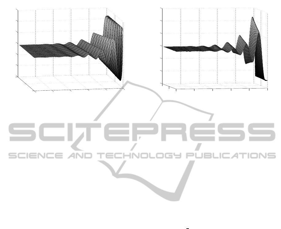
0.5

1.5

2.5

x 10

−3

−1.5

−1

−0.5

0.5

1.5

time [sec]

x ∈ [0, 1]

(t,x) [m/sec]

Figure 3: 3D representation of the forward wave r1(t, x) for

g(t) = 0, f(t, x) = 0 and ICs (50).

= [ ξ

... ξ

z ξ

N−1

... ξ

]. (48)

This arrangement will give different output feedback

cloning template T

and the dynamics for the cells

with nonlinear entries will be described by

˙y

N+1

(t) =



1 −d 0







p(y

N+1

)

N+2





˙y

N+2

(t) =



s −2sd −s 0 0









p(y

N+1

)

N+2

N+3

N+4







(49)

with T

N+1

= T

N+2

= 0, I

N+1

= I

N+2

= 0.

Let us observe that for the ﬁrst proposed arrange-

ment, described by the state vector (42), the matrix

for the linear block – the CNN matrix – has the form

of a circulant matrix.

5 SIMULATION RESULTS

The results of the simulations allow us to verify the

efﬁciency of the numerical technique, to validate the

theoretical results and to understand the physical phe-

nomenon of the propagation of longitudinal vibra-

tions along an elastic rod with boundary constraints

and initial conditions described in (8) and Figure 1.

The simulations were performed for the approxi-

mating system of ODEs (36). The initial value prob-

lem was numerically solved in MATLAB making

use of the CNN structure induced by the state vec-

tor (39). In this manner the interconnection matrix

0.5

1.5

2.5

x 10

−3

−1.5

−1

−0.5

0.5

1.5

time [sec]

x ∈ [0, 1]

(t,x)[m/sec]

Figure 4: 3D representation of the backward wave r2(t,x)

for g(t) = 0, f (t, x) = 0 and ICs (50).

was found to be an almost bi-diagonal lower ma-

trix (excepting 2 elements (a

1,2N

and a

2N+1,N

)) with

only 3 entries which do not obey the template T

[ s −s 0]. We have taken advantage of this sparsity

property in order to reduce the computational effort

and storage.

For the simulation purpose, we considered the

following values for the parameters: E = 288 ·

N/m

, ρ = 8 kg/m

, L = 1 m, A = 0.25·10

−4

l = 1.02 m. For the initial conditions, we have taken

into account the situation suggested in (Timoshenko,

1937): the rod “compressed by forces applied at the

ends, is suddenly released of this compression at t =

0”. This led in our case to the following ICs:



(x) = 1+

−ex, x ∈[0, 1], u

(x) = 0

0, otherwise

(50)

with the unit compression e = 2 ·10

−4

. For simula-

tions, the space discretization step h = 1/10 was suf-

ﬁciently small for the convergence of the algorithm

(simulations performed with h=1/200 lead to same re-

sults).

We have selected 8 ﬁgures to show the results

of simulations: Figure 3 – Figure 10. Figures 3, 4,

5 present a space-time evolution of the forward and

backward waves, as well as the velocity v(t,x) for the

following case: the external forces are zero, i.e.g(t) =

0, f(t,x) = 0 and the damping factor k = 2·10

−4

(very

small and of the same order as the time constant of the

system). Taking t ≤ 2.5 ·10

−3

sec, we focus here on

the effects of initial data (50) on the solutions’ evolu-

tion.

Figures 6, 7, 8, 9, 10 focus on the time evolution

of the displacement u(t,x) at the end x = 1 of the rod.

First two plots show the time evolution of u(t, 1) for

g(t) = 0 and k = 2·10

−4

. One can see that the trajec-

tory starts at u = −10

−4

= u

(1) = ξ

(0) and the ef-

ICINCO2014-11thInternationalConferenceonInformaticsinControl,AutomationandRobotics

536

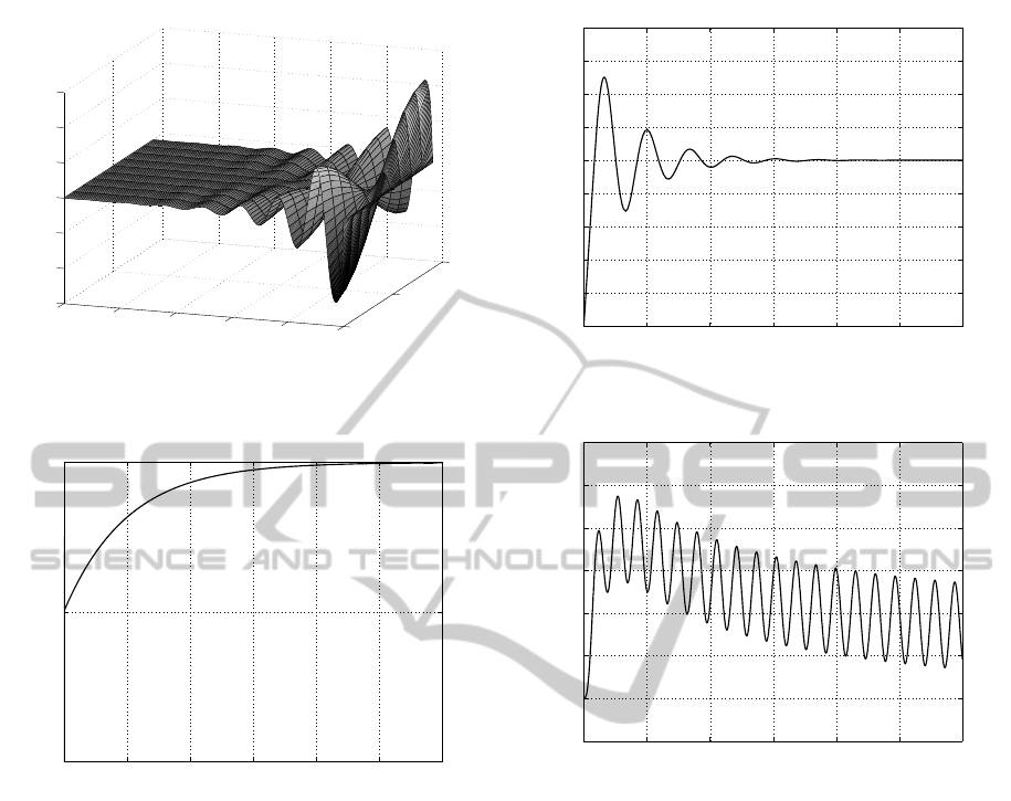
0.5

1.5

2.5

x 10

−3

−1.5

−1

−0.5

0.5

1.5

x ∈ [0,1]

time [sec]

v(t,x) [m/sec]

Figure 5: 3D representation of the velocity v(t, x) for g(t) =

0, f(t, x) = 0 and ICs (50).

0 1 2 3 4 5 6

0.9999

1.0001

time [sec]

u(t,1) [m]

Figure 6: The approximation of the displacement u(t,x) at

x = 1 for g(t) = 0, k = 2·10

−4

fects of the initial conditions vanish after 7 time con-

stants (the settling time being t

= 1.11·10

−3

sec). For

this case, the rod does not interact with the obstacle,

the displacement being smaller than the initial gap.

The last three ﬁgures show the time evolution of

u(t,1) for a time-varying external stimulus g(t) with

f(t, x) = 0 and different values of the damping coef-

ﬁcient. Figures 8 and 9 correspond to the case z > 0,

i.e. the rod interacts with the obstacle at x = 1. They

reveal the cumulated effects of the initial data, stim-

ulus, the nonlinearity p(·) and of the small damping

coefﬁcient related to the amplitude of the stimulus.

These factors lead to additional oscillating modes and

delay the stabilization.

If, on the other hand, the amplitude of the stimu-

lus is not large enough compared to the damping fac-

tor, z < 0 and the rod does not penetrate the obstacle,

which means p(z) = 0. As a consequence, the settling

time is short and the movement of the rod is of the

0 0.5 1 1.5 2 2.5 3

x 10

−3

0.9999

1.0001

time [sec]

u(t,1) [m]

Figure 7: Zoom-in of u(1,t) for g(t) = 0 and k = 2·10

−4

0 5 10 15 20 25 30

0.99

1.01

1.02

1.03

1.04

1.05

1.06

time [sec]

u(t,1) [m]

Figure 8: The approximation of the displacement u(t,x) at

x = 1 for g(t) = 2sin4t, k = 2·10

−4

same type as the reference signal, g(t), as it is shown

in Figure 10.

6 CONCLUSIONS

In this paper we have considered a Mechanical con-

tact problem of an elastic rod with a dashpot attached

to the left end x = 0 and a deformable obstacle with

normal compliance at the opposite extremity x = L.

The rod was subjected to a body force of density f

in the x-direction and to an external force g(t) which

acts at the extremity x = 0. The problem leads to an

one-dimensional hyperbolic equation with boundary

dissipation at one extremity and a regularized con-

tact law at the other extremity. We proved the ex-

istence of weak solutions in the corresponding ﬁnite

energy space H

(0,L)×L

(0,L). In order to approxi-

mate the solution of the problem we used a numerical

technique based on an approach of Method of Lines

NonlinearFeedbackControlandArtificialIntelligenceComputationalMethodsappliedtoaDissipativeDynamicContact

Problem

537

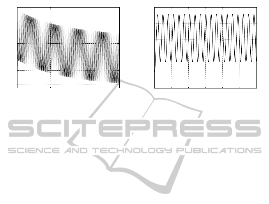
0 50 100 150

0.99

1.01

1.02

1.03

1.04

time [sec]

u(t,1) [m]

Figure 9: u(t,x) at x = 1 for N = 10, g(t) = 5sin4t, k =

8·10

−4

which ensures from the beginning the convergence of

the approximation and the preservation of stability of

the initial problem. Taken into consideration that the

conversion of the mixed initial boundary value prob-

lem for hPDE into an initial value problem leads to

a system of ODEs with a large number of equations

and sparse matrix, the numerical implementation and

simulations employed the CNN paradigm in order to

reduce the computational effort. Considering initial

data of the type encountered in engineering applica-

tions, the results of simulations allowed the visual-

ization of some hidden behaviors for small scales of

time, as well as for long-time behavior.

ACKNOWLEDGEMENTS

This work was partially supported by the grant num-

ber 10C/2014, awarded in the internal grant competi-

tion of the University of Craiova.

REFERENCES

Andersson, L.-E. (1991). A quasistatic frictional problem

with normal compliance. Nonlinear Analysis TMA,

(16):347–370.

Andersson, L.-E. (1995). A global existence result for a

quasistatic contact problem with friction. Advanced

in Mathematical Sciences and Applications, (5):249–

286.

Chua, L. and Roska, T. (1993). The cnn paradigm. IEEE

Trans. Circuits Syst. I, 40(3):147–156.

Danciu, D. (2013a). A CNN Based Approach for Solving

a Hyperbolic PDE Arising from a System of Conser-

vation Laws - The Case of the Overhead Crane, Ad-

vances in Computational Intelligence, volume 7903,

pages 365–374. Springer.

0 5 10 15 20 25 30

0.995

1.005

1.01

1.015

1.02

time [sec.]

u(1,t) [m]

Figure 10: u(t,x) at x = 1 for N = 10, g(t) = 2sin4t, k =

8·10

−4

Danciu, D. (2013b). Numerics for hyperbolic partial dif-

ferential equations (pde) via cellular neural networks

(cnn). In 2nd IEEE Int. Conf. on Systems and

Computer Science ICSCS’2013, pages 183–188, Vil-

leneuve d’Ascq, France.

Danciu, D. and R˘asvan, V. (2014). Delays and Propagation:

Control Liapunov Functionals and Computational Is-

sues, chapter 10. Advances in Delays and Dynamics.

Springer.

Galushkin, A. I. (2010). Neural Network Theory. Springer.

Gilli, M., Roska, T., Chua, L. O., and Civalleri, P. P. (2002).

Cnn dynamics represents a broader class than pdes. I.

J. Bifurcation and Chaos, (10):2051–2068.

Halanay, A. and R˘asvan, V. (1981). Approximations of

delays by ordinary differential equations. Recent ad-

vances in differential equations, pages 155–197.

Han, W. and Sofonea, M. (2002). Quasistatic Contact

Problems in Viscoelasticity and Viscoplasticity. Stud-

ies in Advanced Mathematics 30, American Mathe-

matical Society, Providence, RI—International Press,

Somerville, MA.

Hyman, J. (1979). A method of lines approach to the nu-

merical solution of conservation laws. Advances in

Delays and Dynamics. IMACS Publ. House.

Kikuchi, N. and Oden, J. (1988). Contact Problems in Elas-

ticity: A Study of Variational Inequalities and Finite

Element Methods. SIAM, Philadelphia.

Kim, J. U. (1989). A boundary thin obstacle problem for a

wave equation. Commun. P. D. E., (14):1011–1026.

Klarbring, A. Mikelic, A. and Shillor, M. (1988). Frictional

contact problems with normal compliance. Int. J. En-

gng. Sci., (26):811–832.

Klarbring, A. Mikelic, A. and Shillor, M. (1991). A global

existence result for the quasistatic frictional contact

problem with normal compliance. G. del Piero and F.

Maceri, eds., Unilateral Problems in Structural Anal-

ysis Vol. 4, Birkh¨auser.

Lions, J.-L. (1969). Quelques methodes de resolution

des problmes aux limites non lineaires. Dunod et

Gauthier-Villars, Paris.

ICINCO2014-11thInternationalConferenceonInformaticsinControl,AutomationandRobotics

538

Martins, J. A. and Oden, J. T. (1987). Existence and unique-

ness results for dynamic contact problems with non-

linear normal and friction interface laws. Nonlinear

Analysis TMA, (11):407–428.

Rochdi, M. Shillor, M. and Sofonea, M. (1998). Quasistatic

viscoelastic contact with normal compliance and fric-

tion. Journal of Elasticity, (51):105–126.

Szolgay, P., Voros, G., and Eross, G. (1993). On the ap-

plications of the cellular neural network paradigm in

mechanical vibrating systems. IEEE Trans. Circuits

Syst. I, 40(3):222–227.

Timoshenko, S. (1937). Vibration problems in engineering.

D.Van Nostrand Company.

NonlinearFeedbackControlandArtificialIntelligenceComputationalMethodsappliedtoaDissipativeDynamicContact

Problem

539