A Petri Net Model for an Open Path Multi-AGV System

Davide Giglio

Department of Informatics, Bioengineering, Robotics and Systems Engineering, University of Genova, Genova, Italy

Keywords:

Coloured Petri Nets, Automated Distribution Warehouses, Autonomous Guided Vehicles, Forklift AGVs.

Abstract:

Automated distribution warehouses in which pallet and roll pallet loads are transported by means of forklift

AGVs are considered in this work, with the objective of deﬁning a mathematical model which accurately

represents the behaviour of AGVs in the system. AGVs can move freely in the warehouse (an open path AGV

system is adopted), and their transportation activities can be modelled as a sequence of elementary or basic

actions. In the paper, a coloured Petri net (CPN) model is proposed. It allows representing any sequence of

elementary actions of AGVs (including pick-up and drop-off activities), and accurately models the interactions

among AGVs, in order to guarantee the safety during the execution of activities. The CPN model can be used

to analyse and implement deadlock prevention and deadlock recovery strategies, and it has been adopted in the

building of a discrete-event simulator which is employed to analyse the system’s performance and to evaluate

scheduling policies for transportation tasks.

1 INTRODUCTION

In the last century, the process of automating manu-

facturing systems and other business activities, aimed

at increasing the performance of the systems, has in-

volved both production tasks and transportation op-

erations. In this connection, autonomous guided ve-

hicles (AGVs) have been used to automate the trans-

portation of parts and materials within manufacturing

systems and other indoor or outdoor facilities (Vis,

2006; Le-Ahn and De Koster, 2006). The deﬁni-

tion of an AGV system includes several activities that

can be related to the three standard decision-levels,

namely, the strategic level (layout design), the tactical

level (determination of the number of AGVs, dead-

lock prevention, planning of transportation activities),

and the operational/real-time control level (dispatch-

ing of AGVs, scheduling of transportation activities,

vehicle routing, deadlock avoidance). In this paper,

a mathematical model based on the graphical formal-

ism of the Petri nets (Petri, 1962; Murata, 1989) is

presented; it can be used to solve some of the prob-

lems to be dealt with at the tactical and operational

decision-levels.

In this work, automated distribution warehouses

are taken into account. In the considered class of sys-

tems, the storage area is laid with pallet and roll pallet

loads that must be moved to the gate area when the

trucks which will deliver the items to their ﬁnal des-

tinations arrive at the warehouse. All transportation

activities are carried out by forklift AGVs (Seelinger

and Yoder, 2006; Mart´ınez-Barber´a and Herrero-

P´erez, 2010), which are not constrained to follow

any guide path as they can move freely along the

warehouse’s aisles; then, a free-ranging or open path

model (Sen et al., 1991; Duinkerken et al., 2006) is

adopted. In the system, several AGVs work simul-

taneously (multi-AGV system) and cooperate to par-

allelize the execution of truck loading activities, thus

minimizing the overall completion time.

The management of an open path multi-AGV sys-

tem is of a crucial importance, in particular to guar-

antee the safety during the execution of transportation

activities. Even if vehicles are nowadays equipped

with devices (e.g., lasers) to detect obstacles and other

vehicles, it is necessary to accurately model the move-

ments of AGVs in order to dispatch AGVs, schedule

their activities, and route them in an efﬁcient and safe

way. In this paper, a coloured Petri net (Jensen and

Kristensen, 2009) model, representing all elemen-

tary actions of AGVs (including pick-up and drop-

off activities) and precisely modelling the interactions

among AGVs, is proposed.

The Petri net formalism has been adopted to

model AGVs from the nineties (Holloway and Krogh,

1990; Lee and DiCesare, 1994), and since then Petri

nets have been used to analyse the system’s perfor-

mance, to dispatch AGVs and schedule their activi-

ties, and to analyse and implement deadlock preven-

tion strategies. In (Castillo et al., 2001), the perfor-

734

Giglio D..

A Petri Net Model for an Open Path Multi-AGV System.

DOI: 10.5220/0005054807340745

In Proceedings of the 11th International Conference on Informatics in Control, Automation and Robotics (ICINCO-2014), pages 734-745

ISBN: 978-989-758-040-6

 2014 SCITEPRESS (Science and Technology Publications, Lda.)

AISLE H1A

AISLE H1B

AISLE H2A

AISLE H2B

AISLE H3A

AISLE H3B

AISLE V1A

LE V1B

AISLE V2A

AISLE V2B

AISLE V3A

AISLE V3B

DROP-OFFDROP-OFFDROP-OFF DROP-OFFDROP-OFF DROP-OFF DROP-OFFDROP-OFF

AREAAREAAREA AREAAREA AREA AREAAREA

BUFFER AREABUFFER AREA BUFFER AREABUFFER AREA BUFFER AREABUFFER AREA BUFFE

ER AREA

ATE 2

BUFFER

GATEGATE 1

GATE 3 GATE 4 GATE 5 GATE 7 GATE 9

GATE 1

GATE 4

GATE 5

GATE 7 GATE 9

SHOP 1

SHOP 2

SHOP 3

SHOP 4

SHOP 5

SHOP 6

SHOP 7

SHOP 8

SHOP 9

SHOP 10

SHOP 11

SHOP 12

SHOP 13

SHOP 14

P 15

SHO

SHOP 17

SHOP 18

SHOP 19

SHOP 20

SHOP 21

SHOP 22

SHOP 23

SHOP 24

SHOP 25

SHOP 26

SHOP 27

STORAGE LANE

...

Figure 1: The distribution warehouse.

mance of a tandem AGV system is analysed through

a generalized stochastic Petri net (GSPN) model (Aj-

mone Marsan et al., 1984); deadlock issues are con-

sidered in (Wu and Zhou, 2005), where a maximally

permissivedeadlock avoidance policy is proposed; re-

cently, in (Nishi and Maeno, 2010) and (Nishi and

Tanaka, 2012), Petri nets have been used to dispatch

AGVs and to route them within an AGV system. The

coloured Petri nets has been adopted in (Hsieh, 1998;

Hsieh and Chen, 1999; Dotoli and Fanti, 2004; Aized,

2009) to model, analyse, and simulate AGV systems.

However, in all these works, the considered AGV

systems are guided path, in which AGVs are con-

strained to follow the arcs (generally unidirectional)

of a network representing the available routes/paths

for AGVs in the system.

Instead, in this paper, an open path AGV system

is adopted, since it allows more ﬂexibility in manag-

ing the time-variant AGVs’ tasks that have to be ac-

complished in the considered class of systems. As it

will be described in the following section, AGVs are

required to travel paths which change with time, as

the pick-up and drop-off points change dynamically

on the basis of the trucks’ arrivals and of the assign-

APetriNetModelforanOpenPathMulti-AGVSystem

735

ment of the gates to the trucks; moreover, the vertical

aisles must be traveled by AGVs both in the left side

and in the right side, since the loads to be picked-up

are placed next to both sides of the aisles (see Fig-

ure 1). A guided path system for the considered class

of warehouses would require a very large number of

paths, thus making that kind of approach very com-

plex. Therefore, an open path model is preferred.

This paper is organizedas follows. In section 2 the

class of distribution warehouses and the adopted sys-

tem model are respectively introduced. The coloured

Petri net model is proposed in section 3. Issues about

deadlock prevention and deadlock recovery are dealt

with in section 4, whereas in section 5 some conclud-

ing remarks are reported.

2 THE DISTRIBUTION

WAREHOUSE

In the considered class of warehouses, items to be de-

livered are stacked and stored on pallet and roll pal-

let loads (pallets and rolls, simply), which are placed

on the ﬂoor in short lanes that are physically deﬁned

among the warehouse’s aisles (storage lanes). An ex-

ample of distribution warehouse is illustrated in Fig-

ure 1. Each lane may contain a variable number of

pallets (usually 3 or 4) or rolls (usually 4 or 5), which

are lined up in a row since a lane is about 1 meter

wide. Each storage lane is associated with a “shop”

(e.g., a store or a supermarket) and each shop consists

of one or more consecutive lanes. In general, each

shop holds either pallets or rolls. Shops/lanes are ac-

cessible only through the vertical aisles and only one

side of a storage lane can be approached by the fork-

lift AGVs to get the loads, as illustrated in Figure 1.

Both the horizontal and the vertical aisles are about 3

meters wide, but the horizontal aisle adjacent to the

gate zone, which is wider as it includes the buffer ar-

eas where pallets and rolls, just dropped off by the

forklift AGVs, are temporarily left. Bidirectional traf-

ﬁc of transportation resources is allowed in any aisle,

and AGVs are not required to respect any right-hand

or left-hand rule.

Warehouse activities start each day in the after-

noon and conclude in the morning of the next day.

In the afternoon the orders of stores and supermar-

kets are processed, pallets and rolls are prepared and

moved to the storage lanes corresponding to the shop

to which items have to be delivered (the warehouse is

initially empty). These operations are man-made and

can last up to the evening. In the early morning of the

following day (from about 4 a.m.), trucks arrive at the

distribution warehouse (in accordance with a prede-

ﬁned schedule); each truck has to deliver items to one

or more shops and then pallets and/or rolls are trans-

ported from the storage lanes relevant to those shops

to the buffer area of the gate at which the truck is

parked. A forklift AGV moves to the open side of the

lane, enters the lane horizontally, picks either 1 pallet

or 1 roll or 2 rolls up, exits the lane, travels towards

the relevant gate where it drops the pallet/roll(s) off in

a dedicated zone next to the buffer area of the gate

(drop-off area). This sequence of operations made

by an AGV (empty transfer, pick-up, transportation,

drop-off) represents a single task to be accomplished

by the transportation resource. Activities end when

all pallets and rolls have been delivered.

2.1 The System Model

In order to obtain a system model which allows rep-

resenting the behaviour of AGVs in the distribution

warehouse, the layout (in particular, the horizontal

and the vertical aisles) is divided into cells of approx-

imately the same size (0.8-1 m × 0.8-1 m) so that

a forklift AGV occupies 3 cells when moving in the

warehouse, as illustrated in Figure 2. The position of

a forklift AGV is deﬁned by the cell which is occupied

by the extremities of the forks, and by the direction of

the AGV which is speciﬁed by the “truck” part of it

(then, an AGV has north direction when its forks are

down-side with respect to the truck, has east direction

when its forks are left-side, and so on, for example,

the AGV which is in the aisle V1B has north direc-

tion). The state of a forklift AGV consists of the po-

sition and the load which is transported (no load, 1

pallet, 1 roll, 2 rolls).

An AGV is allowed to execute three kinds of ele-

mentary movements: move straight, rotate 90

◦

, and

turn; they lead to eight “basic actions” which are:

movenorth, move east, move south, movewest, rotate

◦

clockwise, rotate 90

◦

counterclockwise, turn left,

and turn right. A forklift AGV with a certain position

is allowed to perform one or more basic actions (for

example, with reference to Figures 1 and 2, the AGV

which is in the aisle H2A can either move west or

rotate counterclockwise or turn left; turn right is not

allowed since the presence of the corner of the stor-

age lane). All trips, from whichever cell to another

different cell, can be deﬁned as a sequence of basic

actions. Other movements are relevant to the loading

and unloading activities; in this case, a loading action

includes all the basic movements which are necessary

to enter a lane, to place the AGV in the right posi-

tion, to pick the pallet or the roll(s) up, and to exit the

lane; in the same way, an unloading action includes

all the basic movements which are necessary to place

ICINCO2014-11thInternationalConferenceonInformaticsinControl,AutomationandRobotics

736

Figure 2: The system model.

the AGV in the right position and to drop the pallet or

the roll(s) off.

It is worth remarking that the proposed model

can be quite easily enhanced by adding further basic

movements, such as, for example, a diagonal move-

ment to be used to change lane when travelling an

aisle; the new movements would be then modelled

within the CPN representation by following the same

reasoning lines used to model the three kinds of el-

ementary movements here taken into account (de-

scribed in section 3). In any case, the considered ba-

sic movements allows the AGVs to freely travel in the

warehouse, that is, the AGVs can run through an aisle

in any direction and to do that they can stay in the

middle or in any of the side parts of the aisle.

2.2 On Representing the System Model

by means of Coloured Petri Nets

The system model is represented in this paper by

means of coloured Petri nets (CPNs), with the aim

of providing a formal model to be used to analyse the

performanceof the system, to deﬁne deadlock preven-

tion and recovery strategies, and to simulate AGVs

tasks. The choice of using CPNs, instead of (classic)

Petri nets, is due to the need of representing differ-

ent types of loads (pallets and rolls), different states

of the AGV (empty, loaded with 1 pallet, loaded with

1 roll, or loaded with 2 rolls), and different states of

the cells which form the layout. The adopted class of

CPN is the one proposed in (Jensen and Kristensen,

2009), whose deﬁnition is the following.

Deﬁnition 1. A (non-hierarchical) Coloured Petri

Net is a nine-tuple CPN = (P, T, A, Σ, V, C, G, E, I),

where:

1. P is a ﬁnite set of places;

2. T is a ﬁnite set of transitions (P∩ T =

0);

3. A ⊆ P× T ∪ T × P is a set of directed arcs;

4. Σ is a ﬁnite set of non empty colour sets;

APetriNetModelforanOpenPathMulti-AGVSystem

737

5. V is a ﬁnite set of typed variables such that

Type[v] ∈ Σ for all variables v ∈ V;

6. C : P → Σ is a colour set function that assigns a

colour set to each place;

7. G : T → Expr

is a guard function that assigns a

guard to each transition t such that Type[G(t)] =

Bool;

8. E : A → Expr

is an arc expression function that

assigns an arc expression to each arc a such that

Type[E(a)] = C(p)

, where p is the place con-

nected to the arc a;

9. I : P → Expr

is an initialization function that as-

signs an initialization expression to each place p

such that Type[I(p)] = C(p)

In the proposed model, the i-th cell of the layout

is modelled through two places, namely, p

and s

Place p

models the presence of a forklift AGV in the

cell, in particular, the presence of the extremities of

the forks (then, each AGV, even if it physically occu-

pies 3 cells, is represented by a single token moving

through places p

). Place s

represents the state of the

cell, which is deﬁned on the basis of the following

safety-related considerations.

In an open path multi-AGV system, in which

AGVs can move freely in the system layout, safety

is of primary importance. In the proposed system,

safety is guaranteed by assuming that no AGV can

be in any of the cells that are adjacent to the three

occupied by another AGV. In this way, there is al-

ways 0.8-1 meter (at least) between two AGVs. In

Figure 2, the light grey cells surrounding each AGV

are those that cannot be occupied by another AGV. In

other words, an AGV physically occupies three cells

(the dark grey cells) and virtually occupies a maxi-

mum of 12 cells (the light grey ones). Then, before

executing any action or movement, it is always neces-

sary to verify if such a safety constraint is satisﬁed or

not (in this connection, note that cells that are virtu-

ally occupied by an AGV can be also virtually occu-

pied by another AGV). In the rest of the paper, a cell

is:

• “O” (occupied) when it is physically occupied;

• “V” (virtual) when it is virtually occupied;

• “A” (available) if it is neither physically nor virtu-

ally occupied.

Further places of the CPN model are relevant to

the storage lanes and to the drop-off areas. Place l

represents the a-th storage lanes (the marking of l

models the presence of pallets and/or rolls to be trans-

ported), whereas place d

represents the b-th drop-off

area (the marking of d

models the presence of pallets

and/or rolls that are ready to be loaded on the truck).

On the basis of such considerations, the following

sets P, Σ, C, V characterize the proposed CPN model.

P = {p

, s

, l

, d

;

i = 1, . . . , N, a = 1, . . . , L, b = 1, . . . , D}

(1)

being N, L, and D, the number of cells which form the

layout, the number of storage lanes and the number of

drop-off areas/gates, respectively;

Σ = { CELL, LOAD, LTYPE, NO, DIR,

LTYPE× NO× DIR}

(2)

where the colour sets in (2) are deﬁned as

CELL = {O, V, A} (3)

LOAD = {P, R} (4)

LTYPE = {none, P, R} (5)

NO = {0, 1, 2} (6)

DIR = {N, E, S, W} (7)

(P and R stand for pallet and roll, respectively; N, E

S, and W stand for north, east, south, and west, re-

spectively);

C(p

) = LTYPE× NO× DIR i = 1, . . . , N (8)

C(s

) = CELL i = 1, . . . , N (9)

C(l

) = LOAD a = 1, . . . , L (10)

C(d

) = LOAD b = 1, . . . , D (11)

V = {c

: CELL;q : LOAD;l : LTYPE;n : NO;

d : DIR;i = 1, . . . , N}

(12)

The transitions of the CPN represent the execu-

tions of the basic actions. Set T is deﬁned as follows.

T = {t

i− j

, t

i−i

, t

i−a

, t

i−b

;

(i, j) ∈ E , (i, a) ∈ L , (i, b) ∈ D}

(13)

being E , L, and D respectively the set of pairs (i, j)

such that it exists an elementary movement (move

straight or turn) which carries an AGV from the cell i

to the cell j, the set of pairs (i, a) such that the cell i

is next to the storage lane a, and the set of pairs (i, b)

such that the cell i corresponds to the drop-off area b.

Then, transitions of type t

i− j

are relevant to a move

straight or a turn action, those of type t

i−i

are relevant

to a rotate action, whereas transitions of typest

i−a

and

i−b

model respectively a pick-up activity and a drop-

off one.

ICINCO2014-11thInternationalConferenceonInformaticsinControl,AutomationandRobotics

738

3 THE CPN MODEL

The CPN representing the whole system can be ob-

tained by suitably merging the nets representing each

cell. Since the set of actions that an AGV can take de-

pends on the position of the AGV in the system lay-

out, such nets can be different one from another. In

order to generalize the behaviour of an AGV within

a distribution warehouse of the considered class, it is

possible to refer to the generic portion of system lay-

out illustrated in Figure 3, which consists of 121 cells

(11× 11 grid). Such a portion is generic in the sense

that all basic actions (move straight, rotate 90

◦

, and

turn) are allowed for an AGV with the extremities of

the forks in the central cell, namely c

, and having

any direction (the AGV in Figure 3 has north direc-

tion but it is evident that it can have any direction).

100

101

102

103

104

105

106

107

108

109

110

111

112

113

114

115

116

117

118

119

120

121

Figure 3: An AGV in a generic portion of a system layout.

Since every part of the system layout (vertical and

horizontal lanes, X-crossroads, T-crossroads, etc.)

can be “mapped” to such generic portion of the sys-

tem layout, the net representing the behaviour of an

AGV in a speciﬁc cell can be obtained from the

net representing the “meta-cell” c

by removing all

places, transitions, and arcs which are “not involved”,

that is, which refer to cells that are outside of the

“mapped” part. An example relevant to a cell in the

middle-right side of a vertical aisle will be provided

in subsection 3.3.

3.1 Basic Actions

The 5 basic actions (move straight, rotate 90

◦

clock-

wise, rotate 90

◦

counterclockwise, turn left, turn

right) that can be taken by the AGV illustrated in Fig-

ure 3 are now described in detail. The states of the

AGV and of the layout at the start of the movement

are characterized by:

• Start position (cell) of the AGV: c

Start direction of the AGV: north

• O-cells in the layout: c

, c

V-cells in the layout: c

, c

It is worth noting that the 15 further actions that

can be taken by the AGV in c

when its direction is

east or south or west can be easily derived from those

here considered.

3.1.1 Move Straight

This action can be taken only when the cells c

, c

and c

are not O.

START

END

Figure 4: AGV’s behavior in move straight action.

The states of the AGV and of the layout at the end

of the movement are characterized by:

• End position (cell) of the AGV: c

End direction of the AGV: north

• O-cells in the layout: c

, c

V-cells in the layout: c

, c

The states of the cells that have been “released” in

consequence of the movement, namely c

, c

, and

, become either V or A depending on the states of

the cells c

, c

, and c

(for example, c

is V if one of c

, c

is O, and is A otherwise).

3.1.2 Rotate 90

◦

Clockwise

This action can be taken only when cells the c

, c

and c

are A.

START

END

Figure 5: AGV’s behavior in rotate 90

◦

clockwise action.

The states of the AGV and of the layout at the end

of the movement are characterized by:

APetriNetModelforanOpenPathMulti-AGVSystem

739

• End position (cell) of the AGV: c

End direction of the AGV: east

• O-cells in the layout: c

, c

V-cells in the layout: c

, c

The states of the cells that have been released in con-

sequence of the movement, namely c

, c

, and c

, become either A or V depending on the

states of the cells c

, c

, and

(cells c

and c

become A for certain).

3.1.3 Rotate 90

◦

Counterclockwise

This action is very similar to the rotate 90

◦

clockwise

action; the details are not given as they can be eas-

ily derived on the basis of what reported in subsec-

tion 3.1.2.

3.1.4 Turn Left

This action can be taken only when the cells c

, c

and c

are A.

START

END

Figure 6: AGV’s behavior in turn left action.

The states of the AGV and of the layout at the end

of the movement are characterized by:

• End position (cell) of the AGV: c

End direction of the AGV: west

• O-cells in the layout: c

, c

V-cells in the layout: c

, c

The states of the cells that have been released in con-

sequence of the movement, namely c

, c

, and c

, become

either A or V depending on the states of the cells c

, c

, and c

(cells c

, c

, and c

become A for

certain).

3.1.5 Turn Right

This action is very similar to the turn left action; the

details are not given as they can be easily derived on

the basis of what reported in subsection 3.1.4.

3.1.6 Other Actions (Pick-up and Drop-off)

When an AGV is in a vertical aisle, has east or west

direction, and is in a cell next to a storage lane, it can

pick-up a load in the lane (if any) if it is either empty

(in this case it can pick-up either 1 pallet or 1 roll or

2 rolls) or carrying 1 roll (in this case it can pick-up 1

roll). For what concerns the availability (physical or

virtual) of cells, the pick-up activity does not require

speciﬁc conditions to be fulﬁlled as it is assumed that

the cells that are O and V when the activity starts,

remain in their state throughout the execution of the

activity.

Similarly, when an AGV has east or west direction

and is in a cell which corresponds to a drop-offarea, it

can drop-off its load(s). As before, the drop-off activ-

ity does not require speciﬁc conditions on the state of

the near cells (also in this case the cells that are O and

V at the beginning remain in their state throughout the

execution of the activity).

3.2 The CPN Model of the Meta-cell

The coloured Petri net which models all the consid-

ered behaviours of an automatic guided vehicle which

is in cell c

of the 11×11 layout portion represented

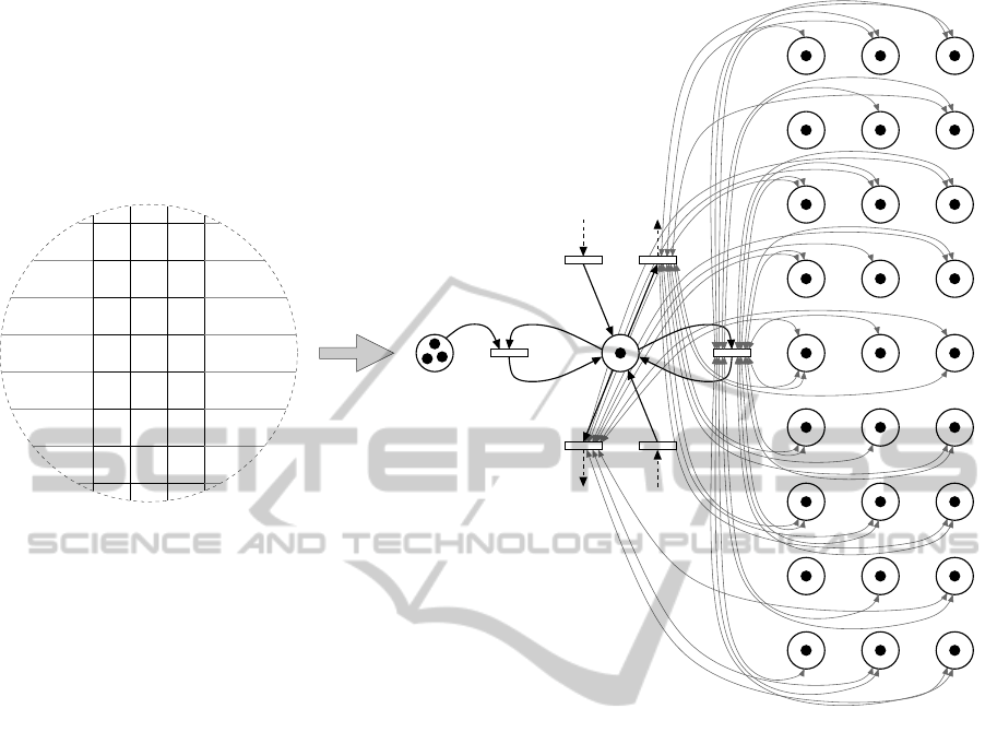
in Figure 3, is illustrated in Figure 7. Such a net is

undoubtedly complex due to the presence of several

arcs. However, in order to evaluate the complexity of

the nets that are generated, it is necessary to take into

account the fact that only a subset of basic actions are

allowed in each of the cells which are present in the

layout of the class of warehouses considered in this

paper (such as the one illustrated in Figures 1 and 2);

this signiﬁcantly reduces the number of transitions.

Moreover, since the aisles are 3 cells wide, the tran-

sitions representing the basic actions will be actually

connected with a reduced number of s

places; this

greatly reduces the number of arcs.

In this connection, in the following subsection the

CPN representing a speciﬁc part in the layout of Fig-

ure 2 (a cell in the middle / right side of the aisle V2A)

is described. It can be derived from the generic one

illustrated in Figure 7 but it has a limited number of

transitions and especially arcs.

Before describing such a simpler net, it is worth

noting that the places representing the state of a cell,

namely s

, i = 1, . . . , N, always contains 1 and only

1 token (or, equivalently, they are safe and always

marked); however, the colour of the token of such

places changes on the basis of the evolution of tokens

through places p

, i = 1, . . . , N, in accordance with the

arc expression function (places p

are safe but not al-

ways marked).

ICINCO2014-11thInternationalConferenceonInformaticsinControl,AutomationandRobotics

740

100

101

102

103

104

105

106

107

108

109

110

112

113

114

115

116

117

118

119

120

106

104

(MOVE NORTH)

(MOVE EAST)

(MOVE SOUTH)

(MOVE WEST)

(TURN LEFT)

(TURN RIGHT)

(ROTATE)

(PICK-UP)

(DROP-OFF)

Figure 7: The CPN model of the meta-cell of the system layout.

3.3 The CPN Model for a Cell in a

Vertical Aisle

The speciﬁc CPN representing a cell in the middle /

right side of a vertical aisle is illustrated in Figure 8.

In such a cell, an AGV can pick-up loads (by ﬁring

transition t

132−71

), rotate (transition t

132−132

), leave

the cell by moving either to north (transition t

132−84

)

or to south (transition t

132−135

). The arc expressions

and the guard function which characterize such ac-

tions are reported in the following subsections (the

arc expressions, which update the state of the cells,

are not discussed for the sake of brevity).

3.3.1 Action: Move North

Arc Expressions

E(p

132

, t

132−84

) = 1

′

(l, n, d)

E(t

132−84

, p

) = 1

′

(l, n, d)

E(s

, t

132−84

) = 1

′

E(t

132−84

, s

) = 1

′

E(s

, t

132−84

) = 1

′

E(t

132−84

, s

) = 1

′

E(s

, t

132−84

) = 1

′

V E(t

132−84

, s

) = 1

′

E(s

130

, t

132−84

) = 1

′

130

E(t

132−84

, s

130

) = 1

′

130

In accordance with (Jensen and Kristensen, 2009), arc

expressions are speciﬁed by using the inﬁx operator

′

which

takes a positive integer as its left argument, specifying the

number of tokens of the colour provided as the right ar-

gument that are removed from (resp., added to) the place

which is the origin (resp., the destination) of the arc.

E(s

132

, t

132−84

) = 1

′

O E(t

132−84

, s

132

) = 1

′

E(s

133

, t

132−84

) = 1

′

133

E(t

132−84

, s

133

) = 1

′

133

E(s

134

, t

132−84

) = 1

′

E(t

132−84

, s

134

) = if (c

130

= O) ∨ (c

133

= O)

∨(c

193

= O) ∨ (c

194

= O) ∨ (c

195

= O) then 1

′

else 1

′

E(s

135

, t

132−84

) = 1

′

E(t

132−84

, s

135

) = if (c

194

= O) ∨ (c

195

= O)

then 1

′

V else 1

′

E(s

193

, t

132−84

) = 1

′

193

E(t

132−84

, s

193

) = 1

′

193

E(s

194

, t

132−84

) = 1

′

194

E(t

132−84

, s

194

) = 1

′

194

E(s

195

, t

132−84

) = 1

′

195

E(t

132−84

, s

195

) = 1

′

195

Guard Function

G(t

132−84

) = (d = N) ∧



6= O) ∧ (c

6= O)



The AGV can move towards north if its direction

is N and if the two cells c

and c

are not physically

occupied.

3.3.2 Action: Rotate

Arc Expressions

E(p

132

, t

132−132

) = 1

′

(l, n, d)

E(t

132−132

, p

132

) = 1

′

(l, n, e)

E(s

, t

132−132

) = 1

′

E(t

132−132

, s

) = 1

′

APetriNetModelforanOpenPathMulti-AGVSystem

741

130

131

132

133

134

135

193

194

195

196

197

198

STORAGE

LANE N. 71

132

84−132

132−84

132−135

135−132

132−132

132−71

130

131

132

133

134

135

193

194

195

196

197

198

199

200

201

FROM

135

Figure 8: Speciﬁc CPN model for a cell in the middle/right side of a vertical aisle.

E(s

, t

132−132

) = 1

′

E(t

132−132

, s

) = 1

′

E(s

, t

132−132

) = 1

′

E(t

132−132

, s

) = 1

′

E(s

, t

132−132

) = select case (d, e): case (N, W) →

′

V; else → 1

′

E(t

132−132

, s

) = select case (d, e): case (N, W) →

if (c

= O) ∨ (c

= O) then 1

′

else 1

′

A; case (W, N) → 1

′

V; else → 1

′

E(s

, t

132−132

) = select case (d, e): case (N, W) →

′

V; else → 1

′

E(t

132−132

, s

) = select case (d, e): case (N, W) →

if (c

= O) ∨ (c

= O) then 1

′

V else 1

′

case (W, N) → 1

′

V; else → 1

′

E(s

, t

132−132

) = select case (d, e): case



(N, W)

∨(W, N)



→ 1

′

A; else → 1

′

E(t

132−132

, s

) = select case (d, e): case



(N, W)

∨(W, N)



→ 1

′

A; else → 1

′

E(s

, t

132−132

) = select case (d, e): case (N, W) →

′

V; case (W, N) → 1

′

A; else → 1

′

E(t

132−132

, s

) = select case (d, e): case (N, W) →

′

A; case (W, N) → 1

′

V; else → 1

′

E(s

, t

132−132

) = select case (d, e): case (N, W) →

′

O; case (W, N) → 1

′

A; else → 1

′

E(t

132−132

, s

) = select case (d, e): case (N, W) →

′

A; case (W, N) → 1

′

O; else → 1

′

E(s

, t

132−132

) = select case (d, e): case (N, W) →

′

A; case (S, W) → 1

′

; else → 1

′

E(t

132−132

, s

) = select case (d, e): case (W, N) →

′

A; case (W, S) → if (c

= O) ∨ (c

= O)

then 1

′

V else 1

′

A; else → 1

′

E(s

, t

132−132

) = select case (d, e): case (N, W) →

′

O; else → 1

′

E(t

132−132

, s

) = select case (d, e): case (W, N) →

′

O; else → 1

′

E(s

130

, t

132−132

) = select case (d, e): case



(N, W)

∨(S, W)



→ 1

′

A; else → 1

′

ICINCO2014-11thInternationalConferenceonInformaticsinControl,AutomationandRobotics

742

E(t

132−132

, s

130

) = select case (d, e): case



(N, W)

∨(S, W)



→ 1

′

O; else → 1

′

E(s

131

, t

132−132

) = select case (d, e): case



(N, W)

∨(S, W)



→ 1

′

V; else → 1

′

E(t

132−132

, s

131

) = select case (d, e): case



(N, W)

∨(S, W)



→ 1

′

O; else → 1

′

E(s

133

, t

132−132

) = select case (d, e): case (N, W) →

′

133

; case (S, W) → 1

′

A; else → 1

′

E(t

132−132

, s

133

) = select case (d, e): case (W, N) →

if (c

193

= O) ∨ (c

194

= O) then 1

′

V else 1

′

case (W, S) → 1

′

A; else → 1

′

E(s

135

, t

132−132

) = select case (d, e): case (S, W) →

′

O; else → 1

′

E(t

132−132

, s

135

) = select case (d, e): case (W, S) →

′

O; else → 1

′

E(s

193

, t

132−132

) = select case (d, e): case



(S, W)

∨(W, S)



→ 1

′

A; else → 1

′

193

E(t

132−132

, s

193

) = select case (d, e): case



(S, W)

∨(W, S)



→ 1

′

A; else → 1

′

193

E(s

194

, t

132−132

) = select case (d, e): case (S, W) →

′

V; case (W, S) → 1

′

A; else → 1

′

194

E(t

132−132

, s

194

) = select case (d, e): case (S, W) →

′

A; case (W, S) → 1

′

V; else → 1

′

194

E(s

195

, t

132−132

) = select case (d, e): case (S, W) →

′

O; case (W, S) → 1

′

A; else → 1

′

195

E(t

132−132

, s

195

) = select case (d, e): case (S, W) →

′

A; case (W, S) → 1

′

O; else → 1

′

195

E(s

197

, t

132−132

) = select case (d, e): case (S, W) →

′

V; else → 1

′

197

E(t

132−132

, s

197

) = select case (d, e): case (S, W) →

if (c

199

= O) ∨ (c

200

= O) ∨ (c

201

= O) then 1

′

else 1

′

A; case (W, S) → 1

′

V; else → 1

′

197

E(s

198

, t

132−132

) = select case (d, e): case (S, W) →

′

V; else → 1

′

198

E(t

132−132

, s

198

) = select case (d, e): case (S, W) →

if (c

200

= O) ∨ (c

201

= O) then 1

′

V else 1

′

case (W, S) → 1

′

V; else → 1

′

198

E(s

199

, t

132−132

) = 1

′

199

E(t

132−132

, s

199

) = 1

′

199

E(s

200

, t

132−132

) = 1

′

200

E(t

132−132

, s

200

) = 1

′

200

E(s

201

, t

132−132

) = 1

′

201

E(t

132−132

, s

201

) = 1

′

201

Guard Function

G(t

132−132

) =



(d = N) ∧ (e = W) ∧



= A)

∧ (c

= A) ∧ (c

130

= A)



∨



(d = W)

∧



(e = N) ∧



= A) ∧ (c

= A)

∧ (c

= A)



∨



(e = S) ∧



193

= A)

∧ (c

194

= A) ∧ (c

195

= A)



∨



(d = S)

∧ (e = W) ∧



130

= A) ∧ (c

133

= A)

∧ (c

193

= A)



The AGV can rotate:

• counterclockwise, from direction N to W, if its

direction is N and if the three cells c

, c

, and

130

are available;

• clockwise, from direction W to N, if its direction

is W and if the three cells c

, c

, and c

are

available;

• counterclockwise, from direction W to S, if its di-

rection is W and if the three cells c

193

, c

194

, and

195

are available;

• clockwise, from direction S to W, if its direction

is S and if the three cells c

130

, c

133

, and c

193

are

available.

3.3.3 Action: Move South

Arc Expressions

E(p

132

, t

132−135

) = 1

′

(l, n, d)

E(t

132−135

, p

135

) = 1

′

(l, n, d)

E(s

, t

132−135

) = 1

′

E(t

132−135

, s

) = 1

′

E(s

, t

132−135

) = 1

′

E(t

132−135

, s

) = 1

′

E(s

, t

132−135

) = 1

′

E(t

132−135

, s

) = 1

′

E(s

, t

132−135

) = 1

′

E(t

132−135

, s

) = 1

′

E(s

, t

132−135

) = 1

′

E(t

132−135

, s

) = if (c

= O) ∨ (c

= O)

∨(c

= O) ∨ (c

130

= O) then 1

′

else 1

′

E(s

, t

132−135

) = 1

′

E(t

132−135

, s

) = if (c

= O) ∨ (c

= O)

then 1

′

V else 1

′

E(s

130

, t

132−135

) = 1

′

130

E(t

132−135

, s

130

) = 1

′

130

E(s

132

, t

132−135

) = 1

′

O E(t

132−135

, s

132

) = 1

′

E(s

198

, t

132−135

) = 1

′

V E(t

132−135

, s

198

) = 1

′

E(s

200

, t

132−135

) = 1

′

200

E(t

132−135

, s

200

) = 1

′

E(s

201

, t

132−135

) = 1

′

201

E(t

132−135

, s

201

) = 1

′

APetriNetModelforanOpenPathMulti-AGVSystem

743

Guard Function

G(t

132−135

) = (d = S) ∧



200

6= O) ∧ (c

201

6= O)



The AGV can move towards south if its direction

is S and if the two cells c

200

and c

201

are not physi-

cally occupied.

3.3.4 Action: Pick-up Pallet/Roll(s)

Arc Expressions

E(l

, t

132−71

) = m

′

E(p

132

, t

132−71

) = 1

′

(l, n, d)

E(t

132−71

, p

132

) = 1

′

(q, n+ m, d)

Guard Function

G(t

132−71

) = (d = W) ∧ (m ≥ 1) ∧



(n = 0)

∧ (l = none) ∧



(m = 1) ∧ (q = P)



∨



(m ≤ 2)

∧ (q = R)



∨



(n = 1) ∧ (l = R) ∧(m = 1)

∧ (q = R)



First of all, the AGV can pick-up loads if its direc-

tion is W, and some loads are present in the storage

lane; moreover, an unloaded AGV can pick-up either

1 pallet or 1 roll or 2 rolls (if available), whereas a

loaded AGV can pick-up 1 roll if its actual load is 1

roll.

4 DEADLOCK ISSUES

Deadlocks may block a multi-AGV system, and such

an issue is indeed critical in open path multi-AGV

systems. In the considered class of systems, some

strategies are taken into account to prevent deadlocks

and to recover from them. However, it is worth not-

ing that this paper is focused on the modelling aspects

of a distribution warehouse; therefore, such strategies

are here only brieﬂy discussed, with no claim of being

exhaustive.

4.1 Deadlock Prevention

The deadlock prevention strategies which are pro-

posed consist, as usually done in this ﬁeld, in apply-

ing some constraints to the behaviour of the forklift

AGVs, so that the probability that two or more AGVs

incur in a deadlock is reduced. The constraints will

be formalized in the CPN as Generalized Mutual Ex-

clusion Constraints (GMEC) which are implemented

by adding some monitor places whose marking either

prevents or allows the ﬁring of transitions, on the ba-

sis of the actual system state.

In the considered class of distribution warehouses,

in which lanes are wide 3 cells, a ﬁrst set of con-

straints for deadlock prevention is the following:

• two AGVs at most can travel in the same aisle

(both horizontal and vertical);

• if two AGVs travel in the same aisle:

– they cannot use the central lane;

– they can use the same lane only if they have

identical direction;

• only one AGV can approach the nine cells of a

crossroad at a time.

Such constraints work well when the number of fork-

lift AGVs is limited (for example, 6-8 AGVs in the

distribution warehouse illustrated in Figures 1 and 2).

However, these deadlock prevention strategies are

not sufﬁcient to guarantee the absence of deadlocks,

since, for example, it can happen that an AGV in

an aisle may require, to complete its turn action, the

room of another aisle which is actually occupied by an

AGV that, in turn, needs to go to the room occupied

by the ﬁrst AGV. For this reason, deadlock recovery

strategies are also considered in the model.

4.2 Deadlock Recovery

The recovery strategy consists in forcing the over-

come of the deadlock situation after a certain amount

of time. This is accomplished by the AGVs which

are assumed to be autonomously able to recover from

a deadlock situation by performing some speciﬁc ac-

tions; when, for example, an AGV encounters another

AGV and a deadlock occurs (because each of the two

AGVs has to go to the room occupied by the other

one), the two AGVs stop their nominal movements

and perform some speciﬁc actions which allow them

to swap their position, thus overcoming the deadlock

situation. Such actions are carried out safely, being

the AGVs equipped with lasers to detect obstacles or

other AGVs.

This capability of AGVs is modelled into the CPN

by adding some net structures (places, timed transi-

tions, and arcs) which recover deadlocks after the esti-

mated amount of time. In particular, the added transi-

tions are enabled by the possible deadlock markings;

when a deadlock occurs, one of these transitions is en-

abled and thus can ﬁre; the ﬁring drives the CPN to a

new marking in which the deadlock has been solved.

ICINCO2014-11thInternationalConferenceonInformaticsinControl,AutomationandRobotics

744

5 CONCLUSIONS

A coloured Petri net model of a distribution ware-

house, in which AGVs move pallets and rolls from the

storage area to the gates of the warehouse, has been

described in this paper. The AGV system is open path

and the proposed CPN model is able to represent the

behaviour of a variable number of AGVs which freely

travel on the system layout. To ensure safety, the pro-

posed CPN model includes colours, guards and arc

expressions which constrain each AGV to be at least

0.8-1 meter distant from any other AGV.

This CPN model has been also used to build

a discrete-event simulator of the distribution ware-

house. Such a simulator, implemented in Extend-

Sim, is currently used to test a scheduling procedure

(based on the solution of some mathematical pro-

gramming problems and a heuristic algorithm) aimed

at assigning the AGVs to the trucks which arrive at the

warehouse and sequencing transportation tasks on the

AGVs. Moreover, the use of the proposed CPN model

for determining the actual paths that the AGVs have

to be follow to minimize travel times and to reduce in-

teractions with other AGVs is currently investigated.

ACKNOWLEDGEMENTS

This work has been supported by A.I.R.O.N.E.

project funded by European Union and Regione Lig-

uria (Italy) under POR-FESR 2007/2013. Special

thanks to the partners of the project: Softeco Sismat

SpA, Sogegross SpA, and Genova Robot Srl.

REFERENCES

Aized, T. (2009). Modelling and performance maximization

of an integrated automated guided vehicle system us-

ing coloured Petri net and response surface methods.

Computers and Industrial Engineering, 57(3):822–

831.

Ajmone Marsan, M., Conte, G., and Balbo, G. (1984). A

class of Generalized Stochastic Petri Nets for the per-

formance evaluation of multiprocessor systems. ACM

Transactions on Computer Systems, 2(2):93–122.

Castillo, I., Reyes, S. A., and Peters, B. A. (2001). Model-

ing and analysis of tandem AGV systems using gener-

alized stochastic Petri nets. Journal of Manufacturing

Systems, 20(4):236–249.

Dotoli, M. and Fanti, M. (2004). Coloured timed Petri net

model for real-time control of automated guided vehi-

cle systems. International Journal of Production Re-

search, 42(9):1787–1814.

Duinkerken, M. B., ter Hoeven, T., and Lodewijks, G.

(2006). Simulating the operational control of free

ranging AGVs. In Perrone, L. F., Wieland, F. P., Liu,

J., Lawson, B. G., Nicol, D. M., and Fujimoto, R. M.,

editors, Proceedings of the 2006 Winter Simulation

Conference, pages 1515–1522.

Holloway, L. E. and Krogh, B. H. (1990). Synthesis of feed-

back control logic for a class of controlled Petri nets.

IEEE Transactions on Automatic Control, 35(5):514–

523.

Hsieh, S. (1998). Synthesis of AGVS by coloured-timed

Petri nets. International Journal of Computer Inte-

grated Manufacturing, 11(4):334–346.

Hsieh, S. and Chen, Y.-F. (1999). AgvSimNet: A

Petri-net-based AGVS simulation system. Interna-

tional Journal of Advanced Manufacturing Technol-

ogy, 15(11):851–861.

Jensen, K. and Kristensen, L. M. (2009). Coloured Petri

Nets. Springer.

Le-Ahn, T. and De Koster, M. B. M. (2006). A review of de-

sign and control of automated guided vehicle systems.

European Journal of Operational Research, 171:1–

23.

Lee, D. Y. and DiCesare, F. (1994). Integrated schedul-

ing of ﬂexible manufacturing systems employing au-

tomated guided vehicles. IEEE Transactions on In-

dustrial Electronics, 41(6):602–610.

Mart´ınez-Barber´a, H. and Herrero-P´erez, D. (2010). Au-

tonomous navigation of an automated guided vehicle

in industrial environments. Robotics and Computer-

Integrated Manufacturing, 26:296–311.

Murata, T. (1989). Petri Nets: Properties, analysis and ap-

plications. Proceedings of the IEEE, 77(4):541–580.

Nishi, T. and Maeno, R. (2010). Petri net decomposition

approach to optimization of route planning problems

for AGV systems. IEEE Transactions on Automation

Science and Engineering, 7(3):523–537.

Nishi, T. and Tanaka, Y. (2012). Petri net decomposition

approach for dispatching and conﬂict-free routing of

bidirectional automated guided vehicle systems. IEEE

Transactions on Systems, Man, and Cybernetics Part

A:Systems and Humans, 42(5):1230–1243.

Petri, C. A. (1962). Kommunikation mit Automaten. Bonn:

Institut f¨ur Instrumentelle Mathematik, Schriften des

IIM Nr. 2.

Seelinger, M. and Yoder, J.-D. (2006). Automatic visual

guidance of a forklift engaging a pallet. Robotics and

Autonomous Systems, 54:1026–1038.

Sen, A., Wang, C., Ristic, M., and Besant, C. (1991). The

supervisory system of the imperial college free rang-

ing automated guided vehicle project. In Proceedings

of the 1991 IEEE International Conference on Sys-

tems, Man, and Cybernetics, pages 1017–1022.

Vis, I. F. A. (2006). Survey of research in the design and

control of automated guided vehicle systems. Euro-

pean Journal of Operational Research, 170:677–709.

Wu, N. and Zhou, M. (2005). Modeling and deadlock avoid-

ance of automated manufacturing systems with multi-

ple automated guided vehicles. IEEE Transactions on

Systems, Man, and Cybernetics, Part B: Cybernetics,

35(6):1193–1202.

APetriNetModelforanOpenPathMulti-AGVSystem

745