
Lip Tracking Using Particle Filter and Geometric Model for Visual
Speech Recognition
Islem Jarraya
1
, Salah Werda
2
and Walid Mahdi
1
1
Multimedia InfoRmation systems and Advanced Computing Laboratory (MIRACL), ISIMS,
University of Sfax, route de Tunis Km 10, Sfax, Tunisia
2
Multimedia InfoRmation systems and Advanced Computing Laboratory (MIRACL), ISGI,
University of Sfax, route de Tunis Km 10, Sfax, Tunisia
Keywords: Lip Localization, Geometric Lip Model, Lip Tracking, Lip Descriptors Extraction, Viseme Classification
and Recognition.
Abstract: The automatic lip-reading is a technology which helps understanding messages exchanged in the case of a
noisy environment or of elderly hearing impairment. To carry out this system, we need to implement three
subsystems. There is a locating and tracking lips system, labial descriptors extraction system and a
classification and speech recognition system. In this work, we present a spatio-temporal approach to track
and characterize lip movements for the automatic recognition of visemes of the French language. First, we
segment lips using the color information and a geometric model of lips. Then, we apply a particle filter to
track lip movements. Finally, we propose to extract and classify the visual informations to recognize the
pronounced viseme. This approach is applied with multiple speakers in natural conditions.
1 INTRODUCTION
Speech is an effective means of communication used
by speakers to understand and exchang messages. In
fact, in noisy environments, the complex message
can be more intelligible and better understood when
it is accompanied by the vision of lip movements; it
is the visual recognition of the speech. Many
researches in the literature investigated their
researches in this context, for example; (Sunil, 2013)
and (Sunil, 2014). They seek to automate lipreading.
Several research works stressed their objectives
in the research on modeling and tracking of the lips
such as; (Mahdi, 2008) , (Cheung, 2011) (Stillittano,
2013) and (Sunil, 2013). Two types of approaches of
segmentation have been used for lipreading: the low-
level approach and The high level approach.
1.1 The Low-Level Approach (Image-
based Approaches)
There are some researches that used the low
segmentation techniques to detect the lip area such
as; (Mahdi, 2008), (Bouvier, 2010), and (Kalbkhani,
2012). These approaches use directly the
information present in the image of the mouth region
and especially the pixel information. In practice,
methods of this type allow rapid locations of the
interest’s zones but can not carry out a precise
detection of the lip edges.
1.2 The High Level Approach
(Model-based Approaches)
There are some researches using the high
segmentation techniques such as; (Mahdi, 2008),
(Liu, 2011), (Stillittano, 2013) and (Sunil, 2013) use
the high level approach to detect the lip area. These
approaches use a deformable model and integrate
regularity constraints. There are two different types
of deformable models which are used; active
contours and parametric models.
1.2.1 Active Contours
There are some researchers that used active contours
such as; (Sunil, 2013) and (Liu, 2011). Active
contour has great flexibility to extract complex
contours. However, when the environmental
conditions are noisy, the detection of the true edge is
not always guaranteed.
172
Jarraya I., Werda S. and Mahdi W..
Lip Tracking Using Particle Filter and Geometric Model for Visual Speech Recognition.
DOI: 10.5220/0005045601720179
In Proceedings of the 11th International Conference on Signal Processing and Multimedia Applications (SIGMAP-2014), pages 172-179
ISBN: 978-989-758-046-8
Copyright
c
2014 SCITEPRESS (Science and Technology Publications, Lda.)
1.2.2 Parametric Models
There are some researchers that used parametric
models such as; (Mahdi, 2008), and (Stillittano,
2013). The main advantage offered by parametric
models is the integration of a priori knowledge about
the shape. This benefit helps the model to converge
good contours.
In order to automatically recognize visemes
(visual phoneme), we must implement a system to
extract relevant visual features on the lips of the
speaker. Therefore, we must develop a system for
locating and tracking mouth to characterize the lip
movements.
This paper is organized as follows. Section (1)
includes the introduction. In section (2), we are
going present our proposed method. Section (3) will
contains the evaluation of the concerned method and
we present our rates of viseme recognition. Finally,
section (4) is for the conclusion.
2 PROPOSED METHOD
We followed the same stages as proposed by
(Mahdi, 2008) for the recognition of visemes, so our
proposed method contains three successive stages.
The first stage includes the lip localization. In the
second stage we use the particle filter for lip
tracking. The third stage we extracted the visual
descriptors for the recognition of visemes.
In this paper tracking the movements of the lips
is the principal objective. In fact, we need to
consider a state vector p
t
compound of parameters
that characterize the state of the initial object. To
make this vector, it is necessary to locate and
segment the lips in the step of initialization at time
t=0.
2.1 Localization of the Closed Mouth
We use two successive thresholding to localize the
mouth. The first threshold is applied to detect the
region of the face. The second threshold is applied to
detect the region of the mouth.
According to (Beaumesnil, 2006), the Red
component is always predominant whatever the
color of the skin. Thus, we used the RGB space to
detect the face and lip areas. But, the presence of the
light in this space is very high. Actually, the
normalization of the RGB space by the luminance
component Y reduces the effect of light in the
image. We tested two different equations luminance
defined by the equation (1) and equation (2) (Mahdi,
2008).
Y1 = R + G + B (1)
Y2 = 0.299 * R + 0.587 G + 0.114 * B (2)
The first thresholding is to detect pixels that
contain the dominance of the Red component
compared to the Green and Blue components in the
normalized image R
n
G
n
B
n
. This is summarized in
the following program:
if ( R
n
(i,j) > G
n
(i,j) et R
n
(i,j) >
B
n
(i,j))
P(i,j) = 0
else
P(i,j) = 255
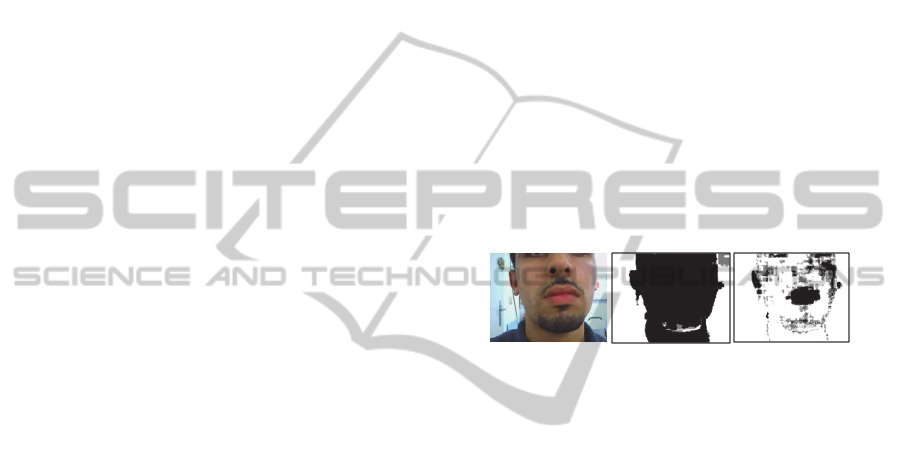
The result obtained by thresholding is presented
in Figure 1.
(a) (b) (c)
Figure 1: Face detection; (a) Source image, (b) Facial area
after thresholding and normalization with Y1, (c) Facial
area after thresholding and normalization with Y2.
The difference between the Red and Green
components is greater for the lips than the skin
(Nicolas, 2003). Thus, we think that this difference
can be a chromatic variable X
i
=(R
n
- G
n
)
i
used for
segmenting lips (i is the number of pixels of the
facial area).
In Figure 2, we show the variation of the
difference between the two components Red and
Green of the facial area. We define a dynamic
threshold to detect only the areas that correspond to
the upper part of the great peaks of the curve where
the Red color is more dominant (equation (3) with
X
: The average of all X
i
, δX
: Deviation of all X
i
).
Figure 2 illustrates the detection of these great peaks
with the dynamic threshold.
Threshold X
δX
(3)
The second threshold results a labial localization
(See Figure 3).
We try to clean the result of the last
threshold to move near the true lip area. Thus, we
use a morphological filter in order to delete false
pixels detected in the skin.
LipTrackingUsingParticleFilterandGeometricModelforVisualSpeechRecognition
173
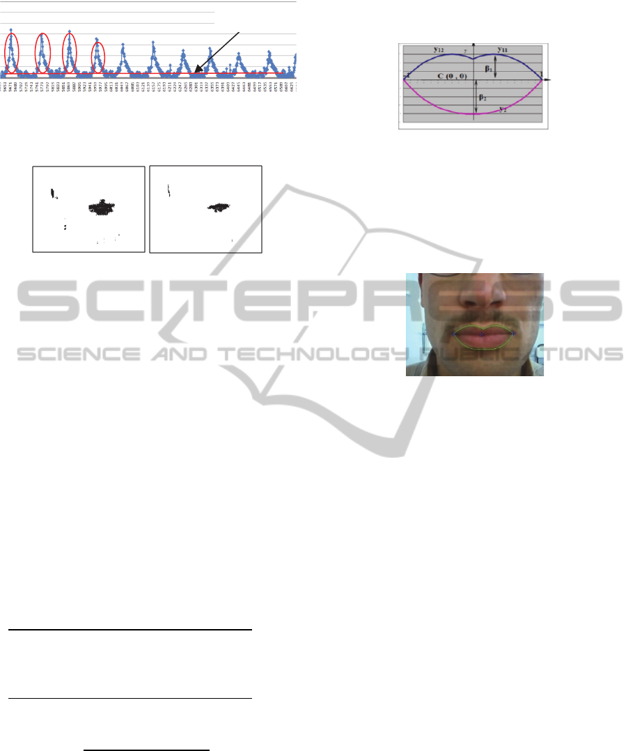
Figure 2: Curve obtained from the difference between the
red color and the green color of the face area.
(a) (b)
Figure 3: Detection lip; (a) the result is obtained after the
application of the second threshold with the image of
Figure 1(b), (b) the result is obtained after the application
of the second threshold with the image of Figure 1(c).
According to (Mahdi, 2008), the corners of the
mouth (right (Cd) and left (Cg)) are defined as the
right and left ends of the center (C) (See Figure 4).
They are detected by using the combination of the
saturation and gradient information. This method of
detection is more explained in (Mahdi, 2008). In
effect, these two corners are the parameters of
initialization, which are used to create a geometric
model that exploits a priori knowledge about the
shape of the lips (Figure 4) (Mahdi, 2008). This
model is composed of three curves: the curve y
11
and
y
12
to trace the contour of the upper lip (Equation
(4), Equation (5)) and the curve y
2
to trace the
contour of the lower lip (Equation (6)).
β
2α
β
x
β
2xα
β
2α
α
2x
β
ε
2
β
α
ε
1
(4)
β
2α
β
x
β
2xα
β
2α
α
2x
β
ε
2
β
α
ε
1
(5)
β
x
∗β
2∗α
∗
β
∗ε
1
(6)
The parameters β, α and ε offer flexibility to
cover the lips (See Figure 4). The β parameter
represents the height of a sub model. The parameter
α describes the degree of curvature of the model.
The ε parameter allows some tolerance for
asymmetrical lips.
Figure 4: Geometric model (Mahdi, 2008).
The tracing of the lip contour is done by creating
a number of possibilities models and selecting the
model that correspond to the most important external
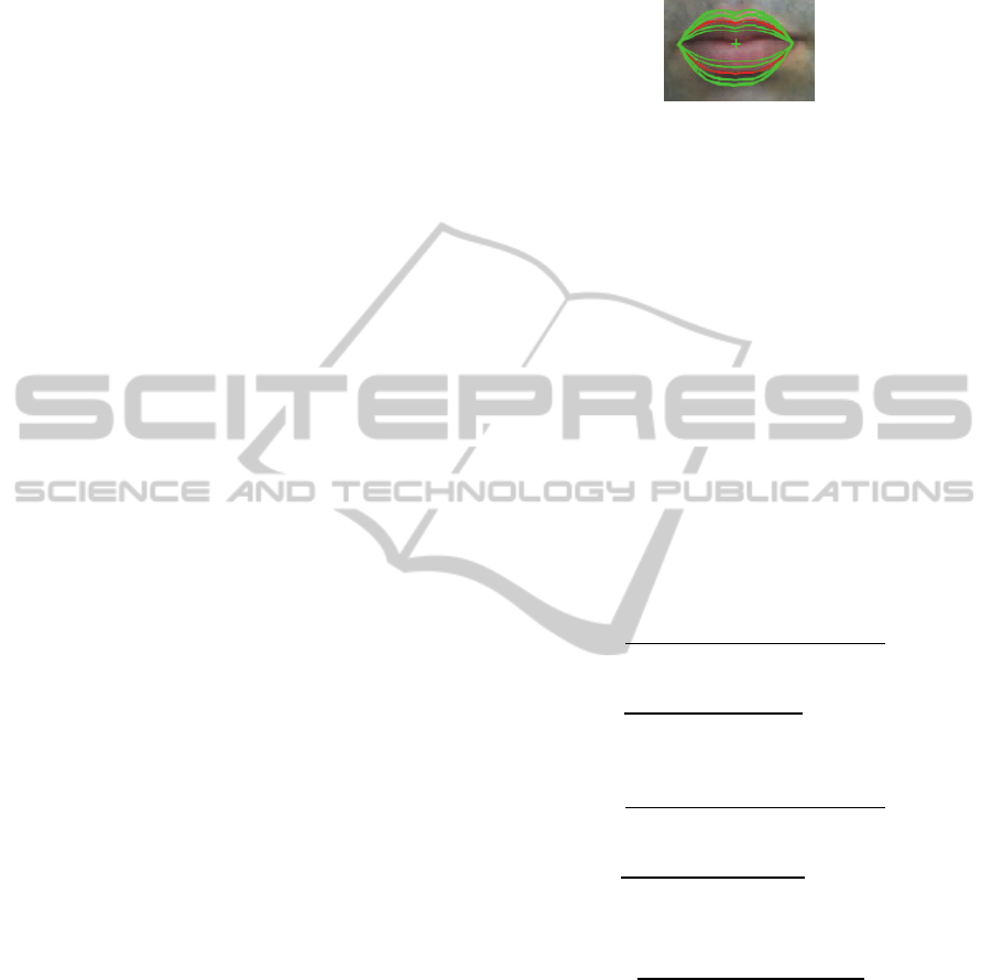
energy of the gradient image (Mahdi, 2008). Figure
5 represents the tracing of the geometric model that
adapts the lip contour.
Figure 5: Lip contour.
2.2 Tracking Lip Contour by the
Geometric Model
The corners are the initialization parameters of the
geometric model. This allows us to propose that
every evolution and deformation of the model are
related to the moving of the corners position over
time. Therefore, lip contour tracking by the
geometric model is linked to corners tracking.
In our case, we use the particle filter for lip
tracking. This filter is a set of advanced predictive
techniques based on simulation. It used in several
works to track a linear or no linear specific object
such as; (Shirinzadeh, 2012), (Majumdar, 2013),
(Segura, 2014) and (Meng, 2014), etc.
2.2.1 Tracking of Corners
Using the particle filter, at time t=0, the two corners
(right C
d
and left C
g
) of the initial geometric model
M
0
are considered as initial objects ((C
0
)
d
and (C
0
)
g
).
Then the state vector “p
t
” of these objects contains
two pose parameters 2D (
,
).
These parameters are the spatial coordinates. Using
the principle of dynamic model P(x
t
|x
t-1
), n of the
predictive corners are created according to equation
(7). (n is experimentally defined)
Threshold
(C)
(C
g
)
(C
d
)
The number of pixel
SIGMAP2014-InternationalConferenceonSignalProcessingandMultimediaApplications
174
(7)
The object “
” has undergone random
transitions by adding a random vector
. This
vector has a normal distribution N(0,K) with a
transitional distance equal to “K” that is
experimentally defined.
In the evaluation step, each particle is defined by
a block of pixel neighborhoods of size N * N pixels.
To calculate the weight of each particle we use the
the manhattan distance between the initial corner
at time “t = 0” and the particle which are shown in
grayscale. This distance measure the degree of
difference between the two intensity vectors of the
neighborhoods pixels of the particle and the pixels
of the initial corner
. Equation (8) defines this
distance (
: the neighborhoods pixels j of the
particle i at time “t”,
: the neighborhoods pixels j
of the initial corner
, the pixel
corresponds the
pixel
).
(8)
Thus, the weight
of the particle
is the
similarity S between the particle and the object
.
The equation (9) defines this measure (
: the
weight of the particle i at time “t”,
: the particle i
at time “t”,
: the initial corner). To estimate the
optimal object, we keep only the ten particles which
have the highest weight. Then, we calculate the
Euclidean distance
|
between the position
of the particle
and the position of the optimal
corner of the time "t-1"
. Thus, the selected
particle has the most similarity (the most weight)
and the smallest Euclidean distance. (Equation (10)).
1/
(9)
1/
|
(10)
2.2.2 Tracking Lip Contour
At time “t=0”, the geometric model that represents
the lip contour M
0
is considered as the initial object.
At each time “t”, using the principle of dynamic
model P(M
t
|M
t-1
), we predict n particles depending
on the selected corners (C
t
)
g
and (C
t
)
d
and the state
of the selected model
at time “t-1” (
is the
optimal model at time “t-1” and n is experimentally
defined) (See Figure 6).
Figure 6: Tracing n particles (green) around the selected
model (red) at time “t-1”.
The coordinates of the two corners right (C
t
)
d
and
left (C
t
)
g
are noted ((x
t
)
d
, (y
t
)
d
) and ((x
t
)
g
, (y
t
)
g
).
Then, generated particles
are linked of poses data
x
,y
with ∈
1,…,
,
∈
,
∀ and
,
,
(Equation (11),
Equation (12), Equation (13), Equation (14)). In fact,
is linked of six parameters
,
,
,
,
et
. Thus, at time “t”, the state
vector of the selected model
is noted by
,
,
,
,
,
.
y
y
y
(11)
y
β
2α
β
x
β
2α
α
2xβ
ε
2xα
β
2β
α
ε
1
(12)
y
β
2α
β
x
β
2α
α
2xβ
ε
2xα
β
2β
α
ε
1
(13)
y
β
x
∗β
2∗α
∗β
∗ε
1
(14)
Each parameter has undergone a random
transformation by adding a random vector
. We
assume that this vector has a normal distribution
N(0,K) with a transitional distance equal to “K” that
is experimentally defined. The transformation of the
parameters is as follows:
,
,
,
,
and
. In point of fact,
,
,
,
,
LipTrackingUsingParticleFilterandGeometricModelforVisualSpeechRecognition
175
and
are parameters of the optimal model
at time “t-1”.
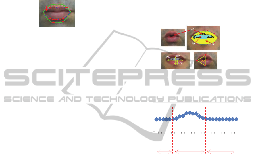
In the evaluation stage, we define m points on the
initial geometric model and their corresponding m
points on each particle. (m is experimentally
defined) In our case m equal 14 (See Figure 7).
Figure 7: Tracing m points on the initial geometric model
(blue) and m points on the particle (green).
Each point is defined by a block of
neighborhoods pixel of size N * N. To calculate the
weight
of each particle, we use the Manhattan
distance D between two intensity vectors of
neighborhoods pixels of the point j (j
∈
[1, ..., m]) of
the initial model and pixels of the corresponding
point in the particle. Thus, the similarity S of a
particle is equal to the inverse of the sum of the
manhattan distances between the m points of the
initial model
and their corresponding points of
the particle
(i
∈
[1, ..., n]) (Equation (15)).
To estimate the optimal object, we keep only the
ten particles which have the highest weight, and we
calculate the Euclidean distance
|
between the position of the particle
(i
∈
[1, ..., n])
and the position of the optimal model of the time "t-
1"
. Thus, the selected particle has the most
similarity (the most weight) and the smallest
Euclidean distance. (Equation (16)).
1/
(15)
1/
|
(16)
2.3 Lip Feature Extraction
The choice of the syllabic descriptors must be
relevant and accurately describe the movement of
each viseme in a corpus. According to (Mahdi,
2008), the most relevant descriptors are visual
descriptors (See Figure 8):
The horizontal distance between lip corners
(DH)
The vertical distance between the lower and
the upper lip (DV’)
The vertical distance between the lower lip and
the centre of the mouth (DV’’)
The degree of the opening mouth (Opening
Degree: OD)
The dark surface (Dark Area: DA) inside the
mouth
The teeth surface (Tooth Area: TA).
In fact, we add two new descriptors (See Figure
8):
The lip surface (Lip Area: LA)
The lip position (Lip Position: LP) (the spatial
position of the lip pixels of the mouth).
Figure 8: Different descriptors characterizing the lip
movements.
Figure 9: Tracking of DV’ with syllable /ba/.
The variation of each descriptor during the
syllabic sequence constructed a data vector. This
vector is the input information in the learning phase
for the visual recognition of the pronounced viseme.
We note that there are two periods of silence at
the beginning and at the end of the speech sequence.
We use DV’ to detect these periods because this
descriptor describes the start and the end of lip
movements (Figure 9). According to (Mahdi, 2008),
the two periods of silence will be ignored for all the
descriptors, in order to not influence the final
recognized template. Then, we propose to apply a
spatial-temporal normalization on the tracking
curves. The normalization is to provide a
representation of the different tracking curves by the
same number of images (w) and in the same range of
values between 0 and 1.
The elocution sequence is captured with 25
frames/s (fps). Moreover, According to (Mahdi,
2008), who used all the frames consecutively for the
0
50
100
1 3 5 7 9 1113151719212325
Distancevalue
Nbimages
DV'
Pause
Pause
The syllable
elocution duration
SIGMAP2014-InternationalConferenceonSignalProcessingandMultimediaApplications
176
duration of 0.4 seconds. Then, in our case, (w) is
fixed to 10.
2.4 Viseme Corpus Presentation
We used the corpus of (Mahdi, 2008). This corpus is
composed of 40 native speakers, of various age and
sex. It has been created in natural conditions. The
capture is done with one CCD camera; the resolution
is 0.35 Mega of pixels and with 25 frames/s (fps).
This cadence is widely enough to capture the major
important lip movement (Mahdi, 2008).
In the French language, we can see three
differentiable lip movements for vowels: group A
(Opening movement), group O (Forward movement)
and group I (Stretch movement). Thus, our corpus
consists of syllable sequences for three visemes
(/ba/, /bi/, /bou/) that are visually differentiable.
These visemes cover three lip movements: /ba/ for
opening /bi/ for stretching and /bou/ for the forward
movement.
3 EXPERIMENTAL RESULTS
We present in this section three experimental parts.
In the first part, we evaluate our lip localization
method, in the second part, we evaluate our lip
tracking method and the third part is used for the
experimentation and the evaluation of our system for
the visual recognition of each viseme present in our
corpus.
3.1 Evaluation of Our Localization
Method
In order to present the result of the location of the
mouth, we draw the detected center of the lip area.
In fact, the step of lip localization is more important
to create the lip contour
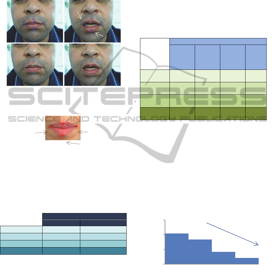
Figure 10: Experimental Results for different speakers
(create the lip contour and detect the four POI “Points Of
Interest: the two corners, the lower point of the lower lip
and the upper point of the upper lip”): (a) results of
(Mahdi, 2008), (b) our results.
If the center of the mouth is bad positioned, the
corners may be poorly positioned and the detection
of the lip contour becomes difficult.
In (Mahdi, 2008) there is a single threshold to
detect the mouth by searching the area where the
Red component is dominant (R
n
> R
n
and G
n
> B
n
).
Figure 10 shows a comparison between the results of
lip localization and lip segmentation with results of
(Mahdi, 2008).
3.2 Evaluation of Our Tracking
Method
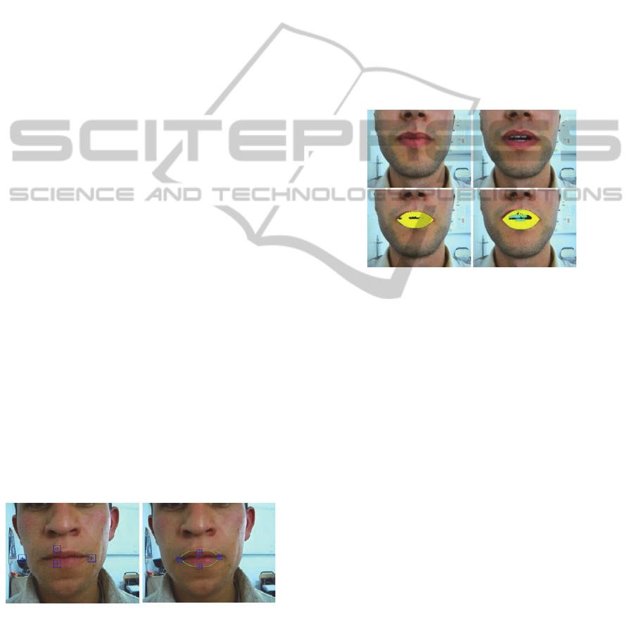
Figure 11 presents the results of tracking and
extracting of the lip movement and the lip
descriptors.
Figure 11: Track and extraction of lip movement and lip
descriptors: pronunciation of the viseme /ba/.
In order to evaluate our tracking method, we
propose to compare our results with the found
results of (Mahdi, 2008). Figure 12 shows a
comparison of some experimental results. The
comparison with found results by the vote algorithm
of (Mahdi, 2008) shows that there is an
improvement in tracking using the particle filter.
In order to properly assess the tracking method,
we try another comparison with manual tracking (a
more real tracking). So, we consider in this part that
the automatic and manual trackings are based on the
evolution of the four points POI of the mouth. The
four POI are the right and left corner, the Up POI
(The upper point of the upper lip) and the Down POI
(the lower point of the lower lip) (Figure 13).
First, we manually detect the positions of the
POI in each frame of 45 sequences using "Matlab
R2010a" software. Then, the position of POI is
automatically calculated again from the automatic
tracking of lip contour. Finally, our tracking method
is evaluated by a comparison between automatic and
manual POI tracking. This comparison is determined
by extracting the mistake of POI tracking. This
mistake is defined by the Euclidean distance
(a)
(b)
LipTrackingUsingParticleFilterandGeometricModelforVisualSpeechRecognition
177
between the POI spatial coordinates which is
determined by using the manual and the automatic
tracking. Tracking errors of 45 sequences are
represented by “Table 1”.
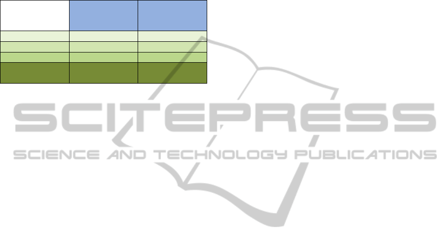
Figure 12: Tracking of lip movement: (a) (b) followed by
vote algorithm of (Mahdi, 2008), (c) (d) followed by our
method (filter particles).
Figure 13: The four points POI of the mouth.
Average errors POIs are varied in the interval
[0.9 pixels, 1.8 pixels] “Table 1”. We note that the
error of tracking is not very important. This argues
the robustness of our tracking method.
Table 1: Tracking error in 45 sequences for three visemes
(/ba/, /bi/ and /bou/).
Error value (pixels)
Average Deviation
Right corner
0,9625 0,5697
Left corner
0,8812 0,6629
Up POI
1,0648 0,6543
Down POI
1,8125 1,2742
3.3 Viseme Recognition
Training and visual recognition require the division
of our audiovisual corpus into two parts. We have
used 70% of the corpus for stage training and 30%
for recognition. We test the recognition percentage
with two types of kernel SVM; the RBF and the
polynomial. The percentage of recognition with the
SVM of RBF kernel is equal to 82.8571% but with
the polynomial kernel we obtain a percentage equal
to 88.5714%. So we choose to represent the found
experimental results with the SVM of polynomial
kernel.
In order to test the utility of the two new
descriptors "LA" and "LP", we test the recognition
rate with four different cases (See “Table 2”).
Table 2: Experimental results found with the SVM of
polynomial kernel and with three different cases of
training.
Recognition Rate
Without
LA and
LP
With
LA and
Without
LP
Without
LA and
with LP
With
LA
and
LP
/Ba/ 58.33% 66.66% 83.33% 91.66
%
/Bi/ 81.81% 81.81%
81.81%
81.81
%
/Bou/ 91.66% 91.66%
91.66%
91.66
%
Recogni-
tion Rate
77.14% 80%
85.71%
88.57
%
In “Table 2”, we note that the descriptors “LA”
and “LP” affect the recognition of the viseme /ba/.
In fact, according to the experimental results, the
rate of confusion of the viseme /ba/ with the viseme
/bi/ is reduced by adding these two descriptors. The
histogram in Figure 14 shows the decrease of this
confusion. Descriptors LA and LP characterize
stretching movement of the lips when pronounce the
viseme /bi/. So this viseme becomes more
identifiable.
Figure 14: Experimental results of viseme confusion.
In order to properly evaluate the recognized
results, the following table shows a comparison with
the results of recognition of (Mahdi, 2008) (See
“Table 3”).
Comparing our results with the results of (Mahdi,
2008), we find that our recognition rates are higher
41,666
33,333
16,666
8,333
0
20
40
60
WithoutLA
andLP
withLAand
WithoutLP
WithoutLA
andwithLP
withLAand
LP
Rateofconfusion
theconfusionoftheviseme/ba/
withtheviseme/bi/
Up POI
Down POI
Right Corner Left Corner
SIGMAP2014-InternationalConferenceonSignalProcessingandMultimediaApplications
178
than recognition rates found by (Mahdi, 2008). This
result shows that our system of tracking and
characterization of lip movements contributes to
improve visual recognition of visemes.
Table 3: Experimental results are found with the SVM of
polynomial kernel and with three different cases of
training.
Recognition
Rate (Mahdi,
2008)
Recognition
Rate (Our
method)
/Ba/ 72.73% 91.66%
/Bi/ 90.91% 81.8181%
/Bou/ 81.82% 91.6666%
Recognition
Rate
81.82% 88.57%
4 CONCLUSIONS
Systems of visual recognition of the speech require
visual descriptors. So, to extract these descriptors, it
is necessary to make a localizing and an automatic
tracking of the labial gestures.
Our objective is to provide a method for
segmenting the labial area and to tracking and
characterizing the lip movements with the best
possible precision to achieve better recognition of
visemes.
In this paper, we presented early our
segmentation method to extract the outer contour of
the lips. Then, we track the lip contour using the
particle filter and extract lip descriptors throughout
the syllable sequence. Finally we chose the SVM
method for training and recognition of visemes. This
approach has been tested with success on our
audiovisual corpus.
Our lip-reading system can be improved by
integrating many new perspectives. In fact, we plan
to expand the content of our corpus by adding others
visemes, different words and even phrases from
different languages. We can also add audio
information.
REFERENCES
Beaumesnil, B., 2006. Real Time Tracking for 3D
Realistic Lip Animation. In ICPR, International
Conference Pattern Recognition. IEEE.
Bouvier, C., 2010. Segmentation Region-Contour des
contours des lèvres. Prepared in the laboratory
GIPSA-lab/DIS within the Graduate School
Electronics, Electrotechnics, Automation & Signal
Processing Laboratory of Computer Vision and
Systems Université Laval.
Kalbkhani, H., Amirani, M., 2012. An Efficient Algorithm
for Lip Segmentation in Color Face Images Based on
Local Information. In JWEET’01, Journal of World’s
Electrical Engineering and Technology. Science-line.
Liu, X., Cheung Y., 2011. A robust lip tracking algorithm
using localized color active contours and deformable
models.In ICASSP, IEEE International Conference on
Acoustics, Speech and Signal Processing.IEEE.
Mahdi, W., Werda, S., Ben Hamadou, A., 2008. A hybrid
approach for automatic lip localization and viseme
classification to enhance visual speech recognition.In
ICAE’03, Integrated Computer-Aided Engineering.
ACM.
Majumdar, J., Kiran, S., 2013. Particle Filter Integrating
Color Model for Tracking. In IJETAE’07,
International Journal of Emerging Technology and
Advanced Engineering.
Meng, J., Liu, J., Zhao, J., Wang, J., 2014. Research of
Real-time Target Tracking Base on Particle Filter
Framework. In Jofcis’06. Journal of Computational
Information Systems. Binary Information Press.
Nicolas, E., 2003. Segmentation des lèvres par un modèle
déformable analytique. Prepared at the Laboratory of
Images and Signals (LIS) within the Doctoral School.
Segura, C., Hernando, J., 2014. 3D Joint Speaker Position
and Orientation Tracking with Particle Filters. In
Sensors’02. Sensors and Transducers Journal. MDPI.
Shirinzadeh, F., Seyedarabi, H., Aghagolzadeh, A., 2012.
Facial Features Tracking Using Auxiliary Particle
Filtering and Observation Model Based on
Bhattacharyya Distance. In IJCTE’05. International
Journal of Computer Theory and Engineering.
EBSCO.
Stillittano, S., Girondel, V., Caplier, A., 2013. Lip contour
segmentation and tracking compliant with lip-reading
application constraints. In Mach. Vis. Appl.’01.
Proceedings of Mach. Vis. Appl. Springer-Verlag.
Sunil, M., Patnaik, S., 2013. Automatic Lip Tracking and
Extraction of Lip Geometric Features for Lip Reading.
In IJMLC’02. International Journal of Machine
Learning and Computing. IACSIT.
Sunil, M., Patnaik, S., 2014. Lip reading using DWT and
LSDA. In IACC. IEEE International Advance
Computing Conference . IEEE.
LipTrackingUsingParticleFilterandGeometricModelforVisualSpeechRecognition
179
