Evolutionary Tuning of Optimal Controllers for Complex Systems

Jesús-Antonio Hernández-Riveros, Jorge-Humberto Urrea-Quintero and Cindy Carmona-Cadavid

Facultad de Minas,Universidad Nacional de Colombia, Cra. 80 No. 65-223, Medellín, Antioquia, Colombia

Keywords: PID Tuning, Heuristic Algorithm, Integral Performance Criterion, Multidynamics Optimization.

Abstract: The Proportional Integral Derivative controller is the most widely used industrial device for monitoring and

controlling processes. Although there are alternatives to the traditional rules of tuning, there is not yet a

study showing that the use of heuristic algorithms it is indeed better than using the classic methods of

optimal tuning. Current trends in controller parameter estimation minimize an integral performance

criterion. In this paper, an evolutionary algorithm (MAGO - Multidynamics Algorithm for Global

Optimization) is used as a tool to optimize the controller parameters minimizing the ITAE (Integral of Time

multiplied by Absolut Error) performance index. The procedure is applied to a set of standard plants

modelled as a Second Order System Plus Time Delay (SOSPD). Operating on servo and regulator modes

and regardless the plant used, the evolutionary approach gets a better overall performance comparing to

traditional methods (Bohl and McAvoy, Minimum ITAE-Hassan, Minimum ITAE-Sung). The solutions

obtained cover all restrictions and extends the maximum and minimum boundaries between them.

1 INTRODUCTION

A comparative study of performance of different

tuning classical methods for PID (proportional-

integral-derivative) controllers is achieved in

(Desanti, 2004). This study concludes that tuning

methods that require a Second Order System Plus

Time Delay model (SOSPD) perform better than

those that require a First Order Lag Plus time Delay

model (FOLPD). O'Dwyer (2009) reports that 90%

of the tuning rules developed are based on a model

of first and second order plus time delay. The most

frequently tuning rules used are not based on an

integral performance criterion. The optimal tuning

rules based on second-order models are just 14 of

the 84 reported until 2009. In general, those rules are

based on several relationships and/or conditions of

the parameters defining the process model. The

SOSPD model was selected in this paper as

representing the plants in order to compare the

performance of a heuristic algorithm with the "best"

techniques developed for PID controllers optimal

tuning. For SOSPD general models 147 tuning rules

have been defined based on the ideal PID structure

(O’Dwyer, 2009).

In (Mora, 2004; Solera, 2006) the performance

and robustness of some tuning rules are evaluated,

and a complete analysis of the methods of tuning

controllers based on SOSPD is made. Each of the

developed tuning rules for PID controllers has only

been applied to a certain group of processes. Usual

tuning methodologies, such as design based on the

root locus, pole-zero cancellation, location of the

closed-loop poles, among others, require

cumbersome procedures and specialized knowledge.

Additionally, most methods for optimal tuning of

SOSPD require extra system information from

experiments carried out directly on the plant;

activities that are not always possible to perform

because the presence of extreme stresses and

oscillations which may create instability and damage

to the system.

The studies mentioned suggest the lack of a

general rule for tuning PID controllers. Due to the

large number of existing tuning rules it is necessary

to find a tuning method that best satisfies the

requirements of each problem and also ensures

optimal values for the controller parameters

according to the selected performance criterion. The

tuning of controllers that minimize an integral

performance criterion can be established as an

optimization problem consisting of minimizing an

objective function.

There is a trend to develop new methods for

tuning PI and PID controllers (Liu, 2001; Solera,

2005; Tavakoli, 2007), posed as a nonlinear

Hernández-Riveros J., Urrea-Quintero J. and Carmona-Cadavid C..

Evolutionary Tuning of Optimal Controllers for Complex Systems.

DOI: 10.5220/0005041100110020

In Proceedings of the International Conference on Evolutionary Computation Theory and Applications (ECTA-2014), pages 11-20

ISBN: 978-989-758-052-9

 2014 SCITEPRESS (Science and Technology Publications, Lda.)

optimization problem. In reviewing the literature is

found that evolutionary algorithms (EA) are applied

to the tuning of controllers on particular cases and

not in the general case as in this paper. Nor are

compared with traditional methods that minimize

some tuning performance index (Chang and Yan,

2004; Junli et al, 2011; Saad et al, 2012a; Saad et al,

2012b). This implies that although there are

alternatives to the traditional rules of tuning, there is

not yet a study showing that the use of heuristic

algorithms it is indeed better than using the

traditional rules of optimal tuning. Hence, this

matter is addressed. Other applications of the EA in

control systems, among them, are system

identification (Hernández-Riveros and Arboleda-

Gómez, 2013) and optimal configuration of sensors

(Michail et al, 2012). The use of an EA for tuning

PID controllers in processes represented by SOSPD

models is proposed in this paper.

This paper is concerned with PID controllers for

processes modeled as SOSPD, optimizing the ITAE

(Integral of Time multiplied by Absolute Error) and

not requiring additional system information.

EA are a proven tool for solving nonlinear

systems and optimization problems. The weaknesses

of these algorithms are in the large number of

control parameters of the EA to be determined by

the analyst and the lack of a solid mathematical

foundation (Whitley, 2001). Looking address these

weaknesses arise recently the Estimation of

Distribution Algorithms, EDA (Lozano, 2006).

These algorithms do not use genetic operators, but

are based on statistics calculated on samples of the

population, which is constantly evolving. This

variant when introduce statistics operators provides

a strong way to demonstrate the evolution.

Nevertheless, they are difficult to manage and do not

eliminate the large number of control parameters of

classical EA. Set a classic EA is itself a difficult

optimization problem; the analyst must try with

probabilities of crossover, mutation, replication,

operator forms, legal individuals, loss of diversity,

etc. Whereas, the EDA require expert skills as the

formulation of simultaneous complex distributions

or the Bayesian networks structure.

For its part, Multi dynamics Algorithm for

Global Optimization (MAGO) also works with

statistics from the evolution of the population

(Hernandez and Ospina, 2010). MAGO is a heuristic

algorithm resulting from the combination of

Lagrangian Evolution, Statistical Control and

Estimation of Distribution. MAGO has shown to be

an efficient and effective tool to solve problems

whose search space is complex (Hernandez and

Villada, 2012) and works with a real-valued

representation. MAGO only requires two parameters

provided by the analyst: the number of generations

and the population size. The traditional EA,

additionally to the number of generations and the

population size requires from the user the definition

of the selection strategy, the individuals’

representation, probabilities of mutation, crossover,

replication, as well as, the crossover type, the locus

of crossing, among others. Depending of its design,

some EA also have extra parameters of tuning as

control variables, number of branch and nodes,

global step size, time constant, etc. (Xinjie and

Mitsuo, 2010). Because of that, MAGO becomes a

good choice as a tool for solving controller tuning as

an optimization problem.

The results obtained by MAGO are compared

with traditional tuning methods not requiring

additional system information. An integral

performance criterion (Integral of Absolute Error –

IAE; Integral of Time multiplied by Absolute Error

–ITAE) is optimized to penalize the error. As it is

further shown, the system model used makes no

difference for the MAGO, because to calculate the

controller parameters only input and output signals

from the closed loop system are required. Regardless

of the relationship between the parameters of the

system (time delay, constant time, etc.) the results

obtained by MAGO overcome those from the

traditional methods of optimal tuning.

This paper begins with an introduction of

controller parameters estimation and performance

index calculation. The tuning of PID controllers on

SOSPD using both the traditional methods and the

evolutionary algorithm MAGO follow. A results

analysis and some conclusions come after.

2 PID CONTROLLER TUNING

The control policy of an ideal PID controller is

shown in equation (1), where E(s) = (R(s) – Y(s)).

The current value Y(s) of the controlled variable is

compared to its desired value R(s), to obtain an error

signal E(s) (feedback). This error is processed to

calculate the necessary change in the manipulated

variable U(s) (control action). Some rules of tuning

controllers are based on critical system information,

on reaction curves and on closed loop tests (

Åström

and Hägglund, 1995).

 

Us Kc TsEs









(1)

ECTA2014-InternationalConferenceonEvolutionaryComputationTheoryandApplications

This paper is concerned to PID controllers for

processes modeled as SOSPD, optimizing the ITAE

and not requiring additional system information.

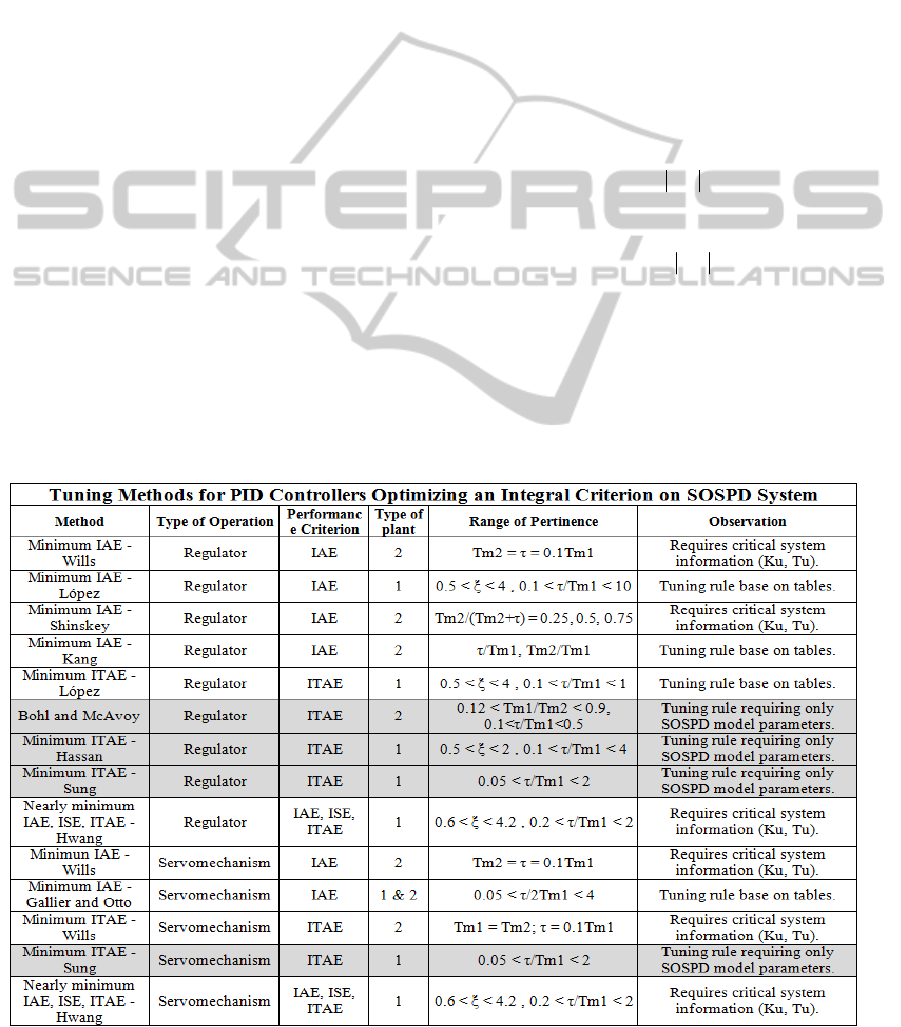
In (O’Dwyer, 2009), it is indicated that 20.7% of

the rules of tuning PID controllers have been

developed from SOSPD models (with or without a

zero in the numerator). This implies 84 rules, 66 of

them do not include the zero in the numerator. Of

these, only 14 optimize an integral performance

criterion, from which 4 rules propose selecting

controller parameters by means of tables and other 6

require additional system information (ultimate gain,

Ku; ultimate frequency, Tu). There are only 4 tuning

rules that optimize an integral performance criterion

and are only function of the SOSPD parameters. For

regulators these rules are: Bohl and McAvoy,

Minimum ITAE - Hassan, Minimum ITAE - Sung;

for servomechanisms: Minimum ITAE - Sung. Table

1 shows the summary of the study, the chosen rules

are shadowed. The equations for the calculation of

proportional gain, Kc; integral time, Ti and

derivative time, Td can be consulted in (Bohl and

McAvoy, 1976; Hassan, 1993; Sung, 1996; Lagunas,

2004). These tuning rules define restrictions on the

behavior of the plant, expressed in the range of

validity.

2.1 Performance Criteria of PID

Controllers

The criterion used for tuning a controller is directly

related to the expected performance of the control

loop. It can be based on desired characteristics of the

response, in time or frequency. Searching for a way

to quantify the behavior of control loops led to the

establishment of performance indexes based on the

error signal, e(t) (feedback). The objective is to

determine the controller setting that minimizes the

chosen cost function. The parameters are optimal

under fixed performance criteria. Of these, the best

known are the so-called integral criteria (

Åström and

Hägglund, 1995), defined in equations (2) and (3).

Integral of Absolute Error

()IAE e t dt







(2)

Integral of Time multiplied by Absolut Error

()ITAE t e t dt







(3)

Where the error is given by:

e(t) = r(t) – y(t) (4)

r(t) is the reference value, and y(t) is the current

value of the controlled variable, both expressed in

time.

Table 1: PID Controller methods requiring only system parameters and minimizing an integral performance criterion.

EvolutionaryTuningofOptimalControllersforComplexSystems

2.2 Plant Parameters and Performance

Indexes

To compare the performance of the studied

controllers it is necessary to tune them with the same

plants. The plant models used are given in equations

(5) and (6) (

Åström and Hägglund, 2000).

()

mmm

Ts Ts











(5)

()

(1 )(1 )

Ts T s









(6)

The following considerations are taken for

equation (5): Kp = 1, τm = 1, ξ = 1 and Tm1 ranging

from 1, 10 and 20. For equation (6), the following

considerations are taken: Kp = 1, τm = 1, Tm1 = 1

and Tm2 = a*Tm1, where a ≤ 1. Table 2 and Table

3 presents a set of transfer functions according to the

parameter values of each plant given by equations

(5) and (6).

Table 2: Transfer Functions of Plants 1, for the tuning.

Plants given by Equation (5)

1_ 1

()

p servo







1_ 1 1_ 1

() ()

p servo p reg

GsGs

1_ 2

()

100 20 1

p servo







1_ 2 1_ 3

() ()

p servo p reg

GsGs

1_ 3

()

400 40 1

pservo







1_ 3 1_ 5

() ()

p servo p reg

GsGs

Table 3: Transfer Functions of Plants 2, for the tuning.

Plants given by Equation (6)

2_ 1

()

(1 )(1 0.1 )

pservo







2_ 1 2_ 1

() ()

p servo p reg

GsGs

2_ 2

()

(1 )(1 0.5 )

p servo







2_ 2 2_ 2

() ()

p servo p reg

GsGs

2_ 3

()

(1 )(1 )

pservo







2_ 3 2_ 3

() ()

p servo p reg

GsGs

The values of the PID controller parameters for

each selected tuning rules are presented, further on,

on Table 4. The parameters are calculated according

to the formulas proposed for each kind of plant. The

selected methods for tuning controllers minimize the

integral performance criterion, ITAE. Therefore, in

Table 4, besides the values of controller parameters,

the ITAE is also reported. The ITAE is calculated in

all cases using the commercial software MATLAB

function "trapz". For the Hassan method, the

controller parameter values are not reported because

there was no convergence in the closed loop system

response for the selected plants given by equation

(5), operating as regulator.

3 TUNING PID CONTROLLERS

USING AN EA

Different solutions there may exist in optimization

problems, therefore a criterion for discriminating

between them, and finding the best, is required. The

tuning of controllers that minimize an integral

performance criterion can be seen as an optimization

problem, inasmuch as the ultimate goal is to find the

combination of parameters Kc, Ti and Td, such that

the value of the integration of a variable of interest is

minimal (error between the actual output of the plant

and the desired value).

EA are widely studied as a heuristic tool for

solving optimization problems. They have shown to

be effective in problems that exhibit noise, random

variation and multimodality. Genetic algorithms, for

example, have proven to be valuable in both

obtaining the optimal values of the PID controller

parameters, and in computational cost (Lagunas,

2004). One of the recent trends in EA is Estimation

of Distribution Algorithms (Lozano et al, 2006).

These do not use genetic operators but are based on

statistics from the same evolving population. The

Multidynamics Algorithm for Global Optimization

(MAGO) (Hernández and Ospina, 2010) also works

with statistics from the evolving population. MAGO

is autonomous in the sense that it regulates its own

behavior and does not need human intervention.

3.1 Optimization and Evolutionary

Algorithms

There are techniques used to obtain better results

(general or specific) for a problem. The results can

greatly improve the performance of a process, which

is why this kind of tools is known as optimization.

When speaking of an optimization problem is to

minimize or maximize depending of the design

requirements.

These mean representative criteria of the system

efficiency. The chosen criterion is called objective

function. The design of an optimization problem is

subject to specific restraints of the system, decision

variables and design objectives, which leads to an

ECTA2014-InternationalConferenceonEvolutionaryComputationTheoryandApplications

expression such that the optimizer can interpret.

Given its nature of global optimizer, an evolutionary

algorithm (EA) is used in this work. EA have been

used in engineering problems (Fleming and

Purshouse, 2002) and the tuning of PID controllers

(Chang and Yan, 2004, Li, 2006). The late is the

case tries in this work, where successful results have

been obtained. The tuning of controllers that

minimize an

objective function can be formulated as

an optimization problem; it is a case of optimal

control (Vinter, 2000). The optimal control consists

in selecting a control structure (including a PID

controller) and adjusts its parameters such that a

criterion of overall performance is minimized. In the

case of a PID controller (equation 1), the ultimate

goal is to find the combination of the Kc, Ti and Td

parameters, given some restrictions, such that the

value of the integral of a variable of interest (error

between the plant’s actual output and the desired

value or control effort) is minimal. The problem

consists of minimizing an objective function, where

its minimum is the result of obtaining a suitable

combination of the three parameters of PID

controller.

3.2 Multidynamics Algorithm for

Global Optimization

MAGO inspires by statistical quality control for a

self-adapting management of the population. In

control charts it is assumed that if the mean of the

process is out of some limits, the process is

Table 4: PID Controller parameters. (NC* = Not converged; B&M*= Bohl and McAvoy).

Plant (2)

PID Operating as Regulator

ITAE

Kc Ti Td

B&M MAGO B&M MAGO B&M MAGO B&M MAGO

P2-reg1

(s)

1.7183 1.4296 1.8978 1.5433 1.8988 0.3341 7.7760 3.1052

P2-reg2

(s)

1.0300 1.4656 1.4164 1.5552 1.6702 0.5597 6.8722 3.6071

P2-reg3

(s)

0.3092 1.8527 0.5854 1.7791 0.7286 0.7575 3.8073 3.6738

Plant (2)

PID Operating as Servomechanism

ITAE

Kc Ti Td

Hassan MAGO Hassan MAGO Hassan MAGO Hassan MAGO

P2-servo1

(s)

N C* 0.5658 N C* 1.6705 N C* 1.0318 NC* 72.6860

P2-servo2

(s)

N C* 0.2731 N C* 1.0966 N C* 0.4871 NC* 69.4943

P2-servo3

(s)

N C* 0.9074 N C* 2.0666 N C* 0.5258 NC* 63.2413

Plant (1)

PID Operating as Servomechanism

ITAE

Kc Ti Td

SUNG MAGO SUNG MAGO SUNG MAGO SUNG MAGO

P1-servo1

(s)

1.2420 1.2318 2.0550 2.1167 0.6555 0.6050 2.0986 2.0486

P1-servo2

(s)

9.0500 10.3237 18.009 16.8942 4.9386 5.5162 3.7911 2.8532

P1-servo3

(s)

16.4953 19.7929 35.689 29.7905 9.5595 10.7718 3.7937 2.7827

Plant (1)

PID Operating as Regulator

ITAE

Kc Ti Td

SUNG MAGO SUNG MAGO SUNG MAGO SUNG MAGO

P1-reg1

(s)

1.8160 1.8557 1.9120 1.7563 0.7073 0.7518 3.8100 3.6623

P1-reg2

(s)

12.8460 17.3252 16.7995 7.4691 -1.99e-6 2.3730 894.5522 3.6427

P1-reg3

(s)

21.8276 31.8262 37.7393 11.0993 -1.17e-4 3.7005 314.5554 4.4240

EvolutionaryTuningofOptimalControllersforComplexSystems

suspicious of being out of control. Then, some

actions should be taken to drive the process inside

the control limits (Montgomery, 2008). MAGO

takes advantage of the concept of control limits to

produce individuals on each generation

simultaneously from three distinct subgroups, each

one with different dynamics. MAGO starts with a

population of possible solutions randomly

distributed throughout the search space. The size of

the whole population is fixed, but the cardinality of

each sub-group changes in each generation

according to the first, second and third deviation of

the actual population. The exploration is performed

by creating new individuals from these three sub-

populations. For the exploitation MAGO uses a

greedy criterion in one subset looking for the goal.

In every generation, the average location and the

first, second and third deviations of the whole

population are calculated to form the groups. The

first subgroup of the population is composed of

improved elite which seeks solutions in a

neighbourhood near the best of all the current

individuals. N1 individuals within one standard

deviation of the average location of the current

population of individuals are displaced in a straight

line toward the best of all, suffering a mutation that

incorporates information from the best one. The

mutation is a simplex search as the Nelder–Mead

method (Xinjie and Mitsuo, 2010) but only two

individuals are used, the best one and the trial one. A

movement in a straight line of a fit individual toward

the best one occurs. If this movement generates a

better individual, the new one passes to the next

generation; otherwise its predecessor passes on with

no changes. This method does not require gradient

information. For each trial individual X

(j)

generation j a shifted one is created according to the

rule in equation (7).

() () () () ()

() () ()

()

jjjjj

Ti Bm

jjj

XXFXX

FSS

 



(7)

Where

()j

is the best individual,

()j

is an

individual randomly selected. To incorporate

information of the current relations among the

variables, the factor F

(j)

depending on the covariance

matrix is chosen in each generation. S

(j)

is the

population covariance matrix at generation j. This

procedure compiles the differences among the best

individuals and the very best one. The covariance

matrix of the current population takes into account

the effect of the evolution. This information is

propagated on new individuals. Each mutant is

compared to his father and the one with better

performance is maintained for the next generation.

This subgroup, called Emergent Dynamics, has the

function of making faster convergence of the

algorithm.

The second group, called Crowd Dynamics, is

formed by creating N2 individuals from a uniform

distribution determined by the upper and lower

limits of the second deviation of the current

population of individuals. This subgroup seeks

possible solutions in a neighborhood close to the

population mean. At first, the neighborhood around

the mean can be large, but as evolution proceeds it

reduced, so that across the search space the

population mean is getting closer to the optimal. The

third group, or Accidental Dynamics, is the smaller

one in relation to its operation on the population. N3

individuals are created from a uniform distribution

throughout the search space, as in the initial

population. This dynamic has two functions:

maintaining the diversity of the population, and

ensuring numerical stability of the algorithm.

The Island Model Genetic Algorithm also works

with subpopulations (Skolicki, 2005). But in the

Island model, more parameters are added to the

genetic algorithm: number of islands, migration size,

migration interval, which island migrate, how

migrants are selected and how to replace individuals.

Instead, in MAGO only two parameters are needed:

number of generations and population size. On

another hand, the use of a covariance matrix to set

an exploring distribution can also be found in

(Hansen, 2006), where, in only one dynamics to

explore the promising region, new individuals are

created sampling from a Gaussian distribution with

an intricate adapted covariance matrix. In MAGO a

simpler distribution is used.

To get the cardinality of each dynamics, consider

the covariance matrix of the population, S

(j)

, at

generation j, and its diagonal, diag(S

(j)

). If Pob

(j)

the set of potential solutions being considered at

generation j, the three groups can be defined as in

equation (8), where: XM(j) = mean of the actual

population. If N1, N2 and N3 are the cardinalities of

the sets G1, G2 and G3, the cardinalities of the

() (())

()

() (())

() 2 (())

() (()), ,

()

() (())

() 2 (())

() 2 (()), ,

()

XM j diag S j x

GxPobj

XM j diag S j

XM j diag S j x

XM j diag S j or

GxPobj

XM j diag S j x

XM j diag S j

XM j diag S j or

GxPobj











 













 



















 



() 2 (())x XM j diag S j











 





(8)

ECTA2014-InternationalConferenceonEvolutionaryComputationTheoryandApplications

Emergent Dynamics, the Crowd Dynamics and the

Accidental Dynamics are set, respectively, and

Pob(j) = G1 U G2 U G3.

This way of defining the elements of each group

is dynamical by nature. The cardinalities depend on

the whole population dispersion in the generation j.

The Emergent Dynamics tends to concentrate N1

individuals around the best one. The Crowd

Dynamics concentrates N2 individuals around the

mean of the actual population. These actions are

reflected in lower values of the standard deviation in

each of the problem variables. The Accidental

Dynamics, with N3 individuals, keeps the population

dispersion at an adequate level. The locus of the best

individual is different from the population’s mean.

As the evolution advances, the location of the best

individual and of the population’s mean could be

closer between themselves. This is used to self-

control the population diversity. Following is

MAGO’s pseudo code.

1: j = 0, Random initial population generation

uniformly distributed over the search space.

2: Repeat

3: Evaluate each individual with the objective function.

4: Calculate the population covariance matrix and the

first, second and third dispersion.

5: Calculate the cardinalities N1, N2 and N3 of the

groups

G1, G2 and G3.

6: Select N1 best individuals, modify them according to

equation (7), make them compete and translate the

winners towards the best one. Pass the fittest to the

generation j + 1.

7: Sample from a uniform distribution in hyper

rectangle [LB(j), UB(j)] N2 individuals, pass to

generation j+ 1.

8: Sample

N3 individuals from a uniform distribution

over the whole search space and pass to generation

j+1

9: j = j + 1

10: Until an ending criterion is satisfied.

3.3 Statement of the Problem

An EA represents a reliable approach when

adjusting controllers is proposed as an optimization

problem (Fleming and Purshouse, 2002). Given their

nature of global optimizers, EA could face non-

convex, nonlinear and highly restrictive optimization

problems (Herreros et al, 2002; Tavakoli et al 2007;

Iruthayarajan and Baskar, 2009). The MAGO has

been shown as a very efficient instrument to solve

problems in a continuous domain (Hernandez and

Villada, 2012). Thus, the MAGO is applied as a tool

for estimating the parameters of a PID controller that

minimizes an integral performance index.

In the case where the system is operating as

servomechanism, the control problem consists of

minimizing the integral of the error multiplied by the

time (ITAE). This involves finding the values for the

parameters Kc, Ti y Td, such that the system gets the

desired r(t) value as fast as possible and with few

oscillations. In the case where the system operates as

a regulator, the reference is a constant R, but the

control problem is also to minimize the ITAE index.

This implies, again, finding the values of the

parameters Kc, Ti and Td, but the goal in this mode

is that at the appearance of a disturbance the system

returns as quickly as possible to the point of

operation. The optimization problem is defined in

equation (9).







(, , )min

cid ITAE

KTT J tetdt







  

(9)

3.4 Evolutionary Design of PID

Controller

The controller design is made for the modes servo

and regulator. For the servo, a change in a unit step

reference is applied. For the regulator, the same

change is applied but as a unit step disturbance to

the second-order plant. The controllers are tuned for

the six plants defined in Table 2 and Table 3. The

two parameters of MAGO: number of generations

(ng) and number of individuals (n), are very low and

fixed for all cases (ng = 150, n = 100). MAGO is a

real-valued evolutionary algorithm, so that the

representation of the individual is a vector

containing the controller parameters. The parameters

are positive values in a continuous domain. See

Table 5.

Table 5: Structure of the EA.

Kc Є R

Ti Є R

Td Є R

The fitness function is in equation (9). The error

is calculated as the difference between the system

output and the reference signal. The error is

calculated for each point of time throughout the

measurement horizon. MAGO does not use genetic

operators as crossover or mutation. The adaptation

of the population is based on moving N1 individuals

to the best one with a Simplex Search, creating N2

individuals over the average location of the actual

population and creating N3 individuals through a

uniform distribution over the whole search space, as

previously discussed.

EvolutionaryTuningofOptimalControllersforComplexSystems

3.5 Controller Parameters and

Performance Indexes

The comparison between the PID controller

parameters obtained with the traditional tuning rules

and the MAGO algorithm are shown in Table 4.

These values minimize the ITAE. Figure 1 illustrates

the time response, in closed loop, for the plants

given in Table 2 and Table 3. Figure 2 illustrates the

time response of the plants defined by equation (6),

given in Table 3. For this mode of operation, in the

literature review, no tuning rule has been found that

could compute the PID controller parameters

requiring only the parameters of the plant. However,

with MAGO is possible to find controller parameters

that minimize the ITAE, without additional

information and regardless of the operating mode.

The closed-loop system simulations from which the

controller was tuned using the MAGO are presented.

4 ANALYSIS OF RESULTS

The study of traditional tuning methods shows that

despite the large amount of available tuning rules,

there is no one that is effective for the solution of all

control problems based on SISO systems. It is

evident that a single tuning rule applies only to a

small number of problems. A tendency to develop

new methods for tuning PID controllers (Tavakoli et

al, 2007; Iruthayarajan and Baskar, 2009; Solera,

2005; Liu and Daley, 2001) has been noticed. The

most recent are focused on controller’s parameter

calculation achieving a desired performance, where

this index is one of those mentioned before (IAE,

ITAE). Table 4 shows the results when tuning PID

controllers for different plant models based on

equations (5) and (6). The parameters obtained

minimize the ITAE criterion. In the case of plants

based on the model of equation (5), when the system

operates as servomechanism, the tuning rules used

are those proposed by Sung. Obtaining an ITAE

close to 3, the response behavior of the system is a

smooth one, free of oscillations (Figure 1).

For the system operating as a regulator the rules

by Sung are employed. In this case the ITAE value

is considerably higher for plants Gp1_servo3 and

Gp1_servo2, and the system presents oscillations.

From this result, it has to be concluded that the rules

proposed by Sung are a good choice for the system

operating as a servomechanism; while for the case

where the system operates as a regulator the use of

these rules should be reconsidered.

On another hand, in the case of plants operating

as regulators, whose model is given by the equation

(6), the rules proposed by Bohl and McAvoy were

used to calculate the controller parameters. The

results for this experiment are reported in Table 4.

The response of the closed loop system is smooth

using the parameters found by this method. The

value for the ITAE performance index, in all cases,

is below 10. Due to the features that the control

problem has, where the objective is to minimize a

function by a suitable combination of controller

parameters which can be expressed as a function of

cost, the solution is presented as an optimization

problem. The algorithm MAGO is used to calculate

the controller parameters seeking to minimize the

ITAE. The results, reported in Table 4, are compared

with those obtained by the traditional tuning rules.

The results obtained by MAGO were very

satisfactory for all cases. The ITAE performance

index is low when the controller parameters are

calculated by the MAGO, whatever the plant is

represented by equation (5) or equation (6), and for

the two modes of operation, servo and regulator.

Additional to the above, the responses of closed loop

systems where the controller parameters are

obtained using the MAGO could be observed in

Figure 1. These responses are softer and exhibit less

oscillation with respect to the response where

controllers are calculated with traditional methods. It

can be appreciate in the Sung case as regulator, that

the addressed problem has a big variability.

Table 4 also reports the results obtained for the

plant based on equation (6). For this case no

comparative data are available, because the only

traditional tuning rule found that minimizes the

performance index ITAE and requires no additional

system information is proposed by Hassan (See

Table 1). However, in the experiments with this

tuning rule it was not possible to obtain convergence

to a real value of the parameters of the controller and

thus it was not possible to calculate the ITAE.

Whereas with MAGO, requiring only the minimum

information of the model, it was possible to find the

controller parameters reaching an acceptable answer,

because in a finite time less than the open-loop

system settling time the reference value is achieved,

see Figure 2.

Figure 1: Response to step change in the input of the plant

(6), as servomechanism (MAGO only).

ECTA2014-InternationalConferenceonEvolutionaryComputationTheoryandApplications

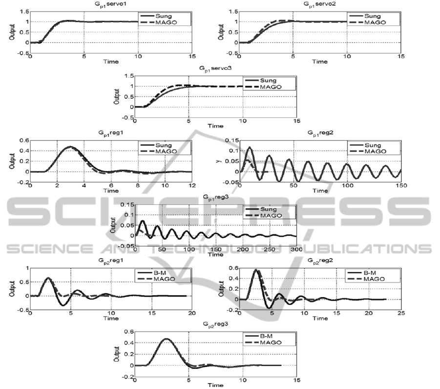
Figure 2: Time response of the plants given by equations (5) and (6), operating as servomechanism and regulator.

5 CONCLUSION

A method of optimal tuning of PID controllers

through the evolutionary algorithm MAGO has been

successfully developed and implemented. The

process resolves the controller tuning as an

optimization problem. The PID controller tuning

was made for SOSPD, without additional knowledge

of the plant. MAGO calculates the parameters of

PID controllers minimizing the ITAE performance

index, and penalizing the error between the

reference value and the output of the plant.

The results showed that MAGO, operating on

servo and regulator modes, gets a better overall

performance comparing to traditional methods (Bohl

and McAvoy (1976), Minimum ITAE - Hassan

(1993), Minimum ITAE - Sung (1996)). Each of

these methods is restricted to certain values on the

behavior of the plant and is limited to an only one

type of operation. The solution obtained with the

evolutionary approach cover all these restrictions

and extends the maximum and minimum between

them. Finally, it should be noted that the MAGO

successful results are obtained regardless of, both,

the plant or controller models used.

ACKNOWLEDGEMENTS

Cindy Carmona-C. was partially supported by the

grant COLCIENCIAS-Jovenes Investigadores 2014.

EvolutionaryTuningofOptimalControllersforComplexSystems

REFERENCES

Åström K. J., Hägglund T., 1995. PID controllers: theory,

design and tuning. Instrument Society of America.

Åström K.J., Hägglund T., 2000. Benchmark Systems for

PID Control. IFAC Workshop on Digital Control --

Past, present, and future of PID Control. Spain.

Bohl A. H., McAvoy T. J., 1976. Linear Feedback vs.

Time Optima Control. II. The Regulator Problem.

Industrial & Engineering Chemistry Process Design

and Development, 15(1), 30-33.

Chang W. D., Yan J. J., 2004. Optimum setting of PID

controllers based on using evolutionary programming

algorithm. Journal of the Chinese Institute of

Engineers, 27(3), 439-442.

Desanti J., 2004. Robustness of tuning methods of based

on models of first-order plus dead time PI and PID

controllers (in Spanish). Escuela de Ingeniería

Eléctrica, Universidad de Costa Rica.

Fleming P. J., Purshouse R. C., 2002. Evolutionary

algorithms in control systems engineering: a survey.

Control Engineering Practice, 10(11), 1223-1241.

Hassan G. A., 1993. Computer-aided tuning of analog and

digital controllers. Control and Computers, 21, 1-1.

Hansen N. (2006). The CMA Evolution Strategy. In:

Towards a new evolutionary computation. Lozano,

Larrañaga, Inza, Bengoetxea, Heidelberg, Springer.

Hernández J. A., Ospina J. D., 2010. A multi dynamics

algorithm for global optimization. Mathematical and

Computer Modelling, 52(7), 1271-1278.

Hernández-Riveros Jesús-Antonio, Villada-Cano Daniel.,

2012. Sensitivity Analysis of an Autonomous

Evolutionary Algorithm. Lecture Notes in Computer

Science. Volume 763. Advances in Artificial

Intelligence. Springer.

Hernández-Riveros J., Arboleda-Gómez A., 2013. Multi-

criteria decision and multi-objective optimization for

constructing and selecting models for systems

identification. Trans.Modelling and Simulation, 55.

Herreros A., Baeyens E., Perán J. R., 2002. Design of

PID-type controllers using multiobjective genetic

algorithms. ISA transactions, 41(4), 457-472.

Iruthayarajan M. W., Baskar S., 2009. Evolutionary

algorithms based design of multivariable PID

controller. Expert systems with Applications, 36(5).

Junli L., Jianlin M.. Guanghui Z., 2011. Evolutionary

algorithms based parameters tuning of PID controller.

Control and Decision Conference, IEEE. 416-420.

Lagunas J. 2004. Tuning of PID controllers using a multi-

objective genetic algorithm, (NSGA-II). (in Spanish)

(Doctoral dissertation) Departamento de Control

Automático. Centro de Investigación y de Estudios

Avanzados. México.

Li, Y., Ang, K.H., Chong, G.C., 2006. PID control system

analysis and design. IEEE Control Systems Magazine

26(1), 32-41.

Liu G. P., Daley S., 2001. Optimal-tuning PID control for

industrial systems. Control Engineering Practice,

9(11), 1185-1194.

Lozano J. A., Larrañaga P., Inza I., Bengoetxea E. (Eds.).

2006. Towards a new evolutionary computation:

Advances on estimation of distribution algorithms.

Springer.

Michail, K., Zolotas, A.C., Goodall, R.M., Whidborne,

J.F., 2012. Optimised configuration of sensors for fault

tolerant control of an electro-magnetic suspension

system, International Journal of Systems Science, 43

(10), 1785-1804.

Montgomery D. C., 2008. Introduction to statistical

quality control. John Wiley & Sons. Wiley, New York.

Mora J. 2004. Performance and robustness of the methods

based on second order models plus dead time tuning

PID controllers. (in Spanish). Escuela de Ingeniería

Eléctrica, Universidad de Costa Rica.

Dwyer A., 2009. Handbook of PI and PID controller

tuning rules (Vol. 2). London: Imperial College Press.

Saad M. S., Jamaluddin H., Darus I. Z. M., 2012a. PID

Controller Tuning Using Evolutionary Algorithms.

WSEAS Transactions on Systems and Control. Issue 4.

Saad M. S., Jamaluddin H., Darus I. Z. M., 2012b.

Implementation of PID controller tuning using

differential evolution and genetic algorithms. Int.

Journal of Innovative Computing Information and

Control, 8(11), 7761-7779.

Skolicki Z., De Jong K., 2005. The influence of migration

sizes and intervals on island models. Proceedings of

the conference on Genetic and evolutionary

computation ACM. 1295-1302.

Solera Saborío E. 2005. PI / PID Controller Tuning with

IAE and ITAE criteria for double pole plants. (in

Spanish). Escuela de Ingeniería Eléctrica, Universidad

de Costa Rica.

Sung S. W., Lee O, J., Lee I. B., Yi S. H. 1996. Automatic

Tuning of PID Controller Using Second-Order Plus

Time Delay Model. Journal of chemical engineering of

Japan, 29(6), 990-999.

Tavakoli S., Griffin I., Fleming P. J., 2007. Multi-

objective optimization approach to the PI tuning

problem. Evolutionary Computation Congress. IEEE.

3165-3171.

Vinter, R., 2000. Optimal Control. Systems & Control:

Foundations & Applications. Springer, London.

Whitley Darrell., 2001. An overview of evolutionary

algorithms: practical issues and common pitfalls.

Information and Software Technology. 43(14).

Xinjie Yu, Mitsuo Gen., 2010. Introduction to

Evolutionary Algorithms. Springer, London.

ECTA2014-InternationalConferenceonEvolutionaryComputationTheoryandApplications