
Modeling & Simulation Framework for the Inclusion of Simulation
Objectives by Abstraction
Sangeeth saagar Ponnusamy
1, 2
, Vincent Albert
2
and Patrice Thebault
1
1
Airbus Operations SAS, 316 Route de Bayonne, 31060, Toulouse, France
2
LAAS-CNRS, 7 Avenue du Colonel Roche, F-31077, Toulouse, France
Keywords: Abstraction, Compatibility, Experimental Frame, Formal Matching, Hybrid Systems, Simulation.
Abstract: Abstractions of experimental frame components with respect to simulation objectives are discussed with a
hybrid system simulation application. Validity assessment through behavioural compatibility criteria
described by the trace inclusion framework is given. The simulation objectives are associated with
modelling abstractions by such a framework and described in established modeling & simulation
framework. Consistent abstractions from hierarchically ordered posets for stimulant and observer models in
experimental frame are discussed. A landing gear example is taken and testability through primary
experimental frame component abstractions was observed for the given simulation requirements. The formal
framework under development is briefly discussed at the end in the context of applicability and derivability
of experimental frame and fidelity of simulation.
1 INTRODUCTION
A system maps input signals to output signals with
an underlying dynamic. Hybrid dynamics in systems
arise out of interaction between continuous
dynamics and discrete dynamics and are found in a
myriad of real world systems, both complex and
simple alike. Modeling and Simulation (M&S) of
such dynamics is difficult due to mutual interaction
of discrete jumps and continuous flows. Abstractions
are always employed in modeling systems and this is
more so true in hybrid systems, however, in
modeling such a system, the choice of abstractions
are crucial to reach the objective of simulation.
However, an abstraction is valid only for a given
validation objective and in (Albert, 2009) validity of
simulation is discussed in terms of class of
abstractions. Abstractions of hybrid systems
especially for safety verification were widely
discussed in (Girard, 2007). Abstraction must
capture the dual relationship between the model and
its intended purpose.
This paper describes the formal approach to
reach this intended objective of simulation through
the abstraction of Experimental Frame (EF)
components described in the established M&S
framework by Zeigler (Zeigler, 1984). The approach
is illustrated with an application to EF abstraction
refinement and verification of a hybrid system
simulation.
2 MODELING ABSTRACTIONS
A model is always an abstraction of reality and in
modeling and simulation of complex systems, often
the difficulty is finding and using consistent and
valid abstractions to model the simulated real world
system with respect to simulation requirement. In
the context of increased usage of simulation as a
means to design and analyse real world complex
systems, a Model-Based Systems Engineering
approach is important in development and usage of
simulation products. This is more so true in
developing a complex simulation product where the
component models are developed by different
stakeholders and a common frame of reference must
exist in terms of implementing consistent
abstractions in the experimental frame.
From systems perspective, consistency is
evaluated through traceability and verification,
whereas validity is evaluated through validation. In a
simulation framework, abstraction of the systems to
simulate the System Under Test (SUT) includes
385
Ponnusamy S., Albert V. and Thebault P..
Modeling & Simulation Framework for the Inclusion of Simulation Objectives by Abstraction.
DOI: 10.5220/0005038903850394
In Proceedings of the 4th International Conference on Simulation and Modeling Methodologies, Technologies and Applications (SIMULTECH-2014),
pages 385-394
ISBN: 978-989-758-038-3
Copyright
c
2014 SCITEPRESS (Science and Technology Publications, Lda.)
abstraction of the stimulant and environmental
systems and this paper deals with the consistency
and validity of stimulant abstractions.
2.1 Experimental Frame
In the context of studying a system through
simulation, the concept of experimental frame
introduced in (Zeigler, 1984) is used to describe
experimental scenarios under which the system and
corresponding models will be used. An EF defines
controllability and observability means to stimulate
and observe the model temporal evolution.
The systems approach in segregating SUT and
EF is often the case in reality when system
development and its validation through simulation
are done by two different entities. The language and
its level of abstraction need to be coherent to derive
any meaningful conclusion from the simulation
results about the real system.
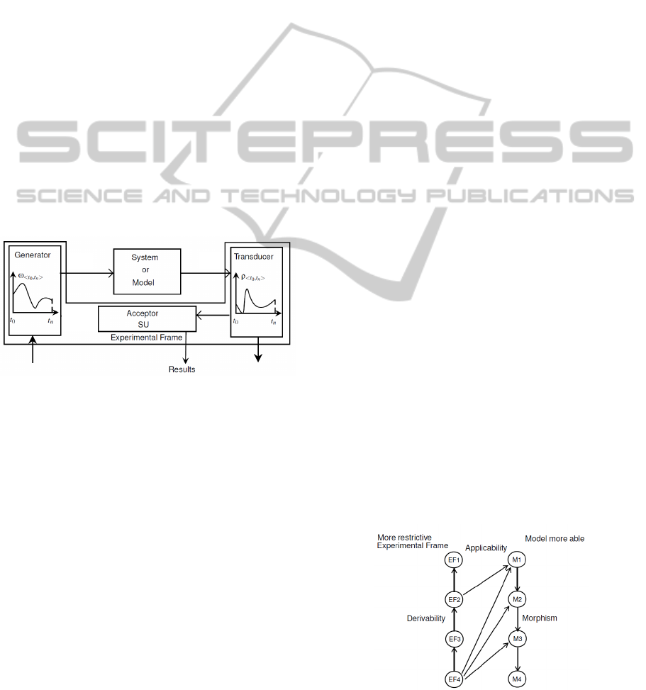
An Experimental Frame, in general, is composed
of a Generator (G), Transducer (T) and Acceptor
(A). A classical illustration of EF as depicted in
(Zeigler, 1984) is shown in the following figure.
Figure 1: Experimental Frame.
Traoré et al defines an EF in the form of following
tuple in (Traoré, 2010)
EF=<T,I
M
,I
E
,O
M
,O
E
, Ω
M
,Ω
E
,Ω
C
, SU>
(1)
where Ω
E
⊆(T,I
E
), Ω
C
⊆T,O
M
and Ω
M
⊆(T,I
M
)
with T is the time base
I
M,E
are the input variable of model and EF
O
M,E
are the output variable of model and EF
Ω
M
are the set of segments injected onto the model
inputs
Ω
E
are the set of admissible input segments for the
experimental control
Ω
C
are the set of segments observed onto the model
outputs
SU is the set of conditions, also referred to as
summary mappings establishing relationship
between inputs and outputs within a frame.
The acceptor dictates the acceptance conditions
for simulation and encoded in temporal logic
Ω
C
⊆T,O
M
⊨ {φ
, φ
…φ
}
(2)
where φ
..
are the requirements defined in a
formalism such as temporal logic. An example could
be, response time for the steady state should be
below a given time limit, φ
=t
sst
< t
limit
.
The generator acts as an input stimulus for the
model, whose outputs are transformed by a
transducer into a comprehensible form, which are in
turn compared against a set of acceptable conditions
specified by an acceptor. In addition, the EF may
contain environmental models which simulate the
real environment in which the SUT operates. Thus
the EF components may be classified broadly as
primary and secondary components with the former
being the prime drivers of simulation, namely
generator, acceptor and transducer, and the latter
being environmental models. The components could
be interconnected and hierarchically composed to
build an EF. However, it must be noted that
abstraction of environmental models are equally
important as such models are seldom absent in an
EF.
2.1.1 EF Applicability & Derivability
In (Albert, 2010), the concepts of homomorphism,
applicability and derivability are discussed in the
framework of M&S. A morphism relation
establishes correspondence between a concrete
model and an abstract model and such a relation
between two models is called homomorphism when
the transition and output function has been preserved
i.e. behavioural equivalence. Applicability and
derivability are more structural concepts in that the
former determines whether an EF can be applied to a
model and the later determines the extent of such an
application. Applicability and derivability defines
compatibility criteria between a model and EF. This
compatibility is influenced by the abstraction level
of EF components and the paper deals with the
Figure 2: Morphism, Applicability & Derivability
relations.
I
M
O
M
O
E
I
E
SIMULTECH2014-4thInternationalConferenceonSimulationandModelingMethodologies,Technologiesand
Applications
386

applicability of such an abstraction. Figure 2, taken
from (Zeigler, 1984), illustrates this concept
between the derivability and hierarchy of
abstractions and the relation between them through
applicability.
2.2 Validity in Experimental Frame
In general, a model is said to be valid if it satisfies
the experimental frame. In this context, in (Albert,
2009), experimental frames were proposed in terms
of model usage domain and objective domain called
Simulation Domain of Use (SDU) and Simulation
Objective of Use (SOU) respectively.
Simulation validity in other words can be defined
as the compatibility between SDU and SOU.
Compatibility, in general, is defined as the degree of
conformity between the considered entities. A valid
simulation has the prerequisite of syntactic and
semantic compatibility between the SDU and SOU.
A study on semantic compatibility between the ports
of simulation models based on ontologies was done
in (Man, 2009). Similarly, in (Albert, 2010),
compatibility between EF and model interfaces were
discussed in terms of syntactics parameters such as
topology, scope, type signature, I/O relation. In this
paper, however, compatibility is discussed in terms
of validity through abstraction. In simulating a
complex system which is hierarchically composed of
different subsystems, modeling abstraction choices
in building a SDU consistent with the simulation
objectives described by SOU will yield this
compatibility. In addition, simulation product
validity is an aggregation of the problem of
correctness and validity. The correctness of
implementation or verification is not discussed here
and only the abstraction influence of primary EF on
validity is discussed.
2.2.1 Primary EF Component Validity
SDU and SOU intuitively refers to model
behavioural limits and model behavioural
expectations respectively. Then the key question is
how to drive the model behaviour to reach its
intended expectations in the context of simulation.
In other words, what are the necessary and
consistent abstractions to be made in the EF
components to drive the SUT to an acceptable
degree of validity? This paper deals with the
reachability of SOU through primary EF component
abstractions. The reachability of SOU through
environmental model abstractions and their
composition with primary components are subject of
another study and are not discussed here.
From the systems perspective, testability of a
system is based on the controllability and
observability of the system components.
Controllability and observability defines the ease of
bringing and propagating data to the input and
output of the component respectively. Thus the
abstraction of primary EF components must result in
adequate testability conditions with respect to the
simulation objectives.
In (Foures, 2013), a method of defining the
intended purpose of simulation for discrete event
simulation of a continuous system was presented by
Damien et al. In (Foures, 2012), a formal
compatibility between EF and FD-DEVS model was
proposed in terms of metrics defined on scope,
precision and state space. The state space metric was
discussed in terms of trace inclusion and a truth table
was proposed to describe the model coverage by EF.
This study is an extension of such definition of SDU
and SOU to simulation of a hybrid system in the
context of input abstraction and its subsequent
compatibility to an EF.
The compatibility is discussed in terms of
reachability of the SUT where reachability is defined
as the set of all possible states reachable by a system
and is used to verify temporal logic properties
defined as safety etc. In this context of definition of
validation requirements, it is important to distinguish
between simulation validity and system validity.
Simulation validity answers whether the simulation
is adequate to answer questions on system
validation. System validation is validation of system
with respect to its requirements. Simulation validity
is a prerequisite of system validity and thus
decisions taken at any stage along the V cycle where
simulation is used as a means of Verification &
Validation, it is intrinsically tied to the key question
of simulation fidelity. A system is said to be valid by
simulation only when the simulation itself is valid
and thus it is a necessary and sufficient condition for
system validity assessment through simulation. Let
φ
and φ
be system and simulation
requirements respectively on the system (S
) and
its representation (S
).
System validation through simulation implies the
acceptor input i.e. model output, satisfies system
requirements and thereby simulation requirements,
⊨φ
⇒⊨φ
(3)
where,
⊨φ
means simulation validity. The
converse may not be true
⊨φ
⊬⊨φ
.
The system validity assessment by simulation
thus becomes
Modeling&SimulationFrameworkfortheInclusionofSimulationObjectivesbyAbstraction
387

φ
i1..n
φ
⋃φ
(4)
In other words, the above equation dictates that
reachability under input stimuli Ω
to the model
from EF (Ω
must result in model output
Ω
satisfying φ
..
to be a valid model.
It may be recalled that the distance between
system and simulation validation is introduced by
abstraction of the system as a simulation model. The
study deals with what are the necessary and
consistent modeling abstractions to be implemented
in simulation such that they are consistent with
system validation requirements. In other words,
choosing abstractions such that the simulation is
adequate i.e. valid to draw any meaningful
conclusion about the real system. Assuming correct
environmental model abstraction, the question is
abstraction of the primary EF components in driving
the simulation to its objective with respect to SDU.
In this paper, through reachability of SUT, necessary
and consistent primary EF abstractions with respect
to system requirements are discussed.
2.2.2 Primary EF Component Abstraction
The primary components of EF are given as
M
p
=<T,X
p
,Y
p
> ∣ p={G,T,A
(5)
where X and Y are input and output variables
defined with over a time base T. Similar to the
general EF definition, we define
Ω
Y
p
⊆(T,Y
p
), are the set of output segments
Ω
X
p
⊆(T,X
p
), are the set of input segments
A morphism relation establishes correspondence
between a concrete model and its abstract version
through abstraction operation. Abstractions are
manyfold depending on the simulation objectives
and hypotheses. From the classes of abstractions
defined in (Albert, 2009), we define abstraction
operation as α over an abstraction class. Such
abstractions are related by binary relations forming a
partial order. A partially ordered set or a poset is a
set P=(≼, S)with reflexive, transitive relation on a
set S. The hierarchy of abstractions could be defined
as a partial order relation over a finite lattice.
M
p
C
α
i
1
→M
p
1
α
i
→…M
p
n
(6)
Different abstraction operations may be feasible
over such a finite lattice whose height is defined by
a set N. The valid set of abstractions among them are
defined by
{α
p
n
} ⊨ {φ
, φ
…φ
} ∣ n ∈N
(7)
In addition to abstraction of model semantics,
model interfaces are abstracted based on their syntax
definition and semantics it handles. The syntactics
(number of ports, coupling, structure) and semantics
(data type, type signature) of EF and SOU interfaces
must be compatible and are defined in terms of a
partial order relation. Such a definition followed by
an inclusion criterion will help address the
simulation validity with respect to abstractions.
The general inclusion relation between the
admissible model input segments with respect to its
capabilities are defined by
Ω
M
SOU
⊆Ω
M
SDU
(8)
It must be noted that there could be interconnection
(i→d) between environmental models and primary
components and the applicability extends to them as
well. In EF definition as a tuple in [Albert, 2010],
the coupling between models M with identifiers I is
given by Z.
EF T,X
EF
,Y
EF
,{M
d
},{I
d
},Z
EF
i→d
(9)
where EFSOU,SDU.
The experimental control segments to model, Ω
E
and
acceptor input, Ω
C
then becomes
Ω
M
Ω
Y
G
⋃Ω
Y
EM→M
Ω
C
Ω
X
T
⋃Ω
X
M→EM
(10)
Acceptance conditions require transduced outputs or
outputs of the SUT or environmental models. The
compatibility is given by
Ω
Y
T
∨ Ω
Y
M
∨ Ω
Y
EM→A
⊆ Ω
X
A
(11)
Utilising such definition, applicability is extended as
Ω
Y
G
⋃Ω
Y
EM→M
⊆ Ω
X
M
Ω
Y
T
⋃Ω
X
M→EM
⊆ Ω
Y
M
(12)
The compatibility criteria described above also
includes model constraints, ∅
M
defined by the
behavioural limits in terms of possible reachable
states (S), in other words SDU, as well as the
constraints on the inputs (X) and outputs (Y).
∅
M
= ∅{X
M
,Y
M
,S
M
}
(13)
Constraints on state, output and input are defined for
all the EF and SUT and violation of such constraints
results in inconsistency. The constraint on the state
evolution is given below
∀S
M
i
→S
M
i1
such that
(S
M
i
,S
M
i+1
∈∅
M
S
M
(14)
Intuitively, the above equation lays out a consistency
SIMULTECH2014-4thInternationalConferenceonSimulationandModelingMethodologies,Technologiesand
Applications
388

criteria such that the under transition relation, , the
evolution of state from step i to i+1 respect the
constraints imposed on the state space. Similarly,
such definition can be extended to inputs and
outputs.
2.3 Model Coverage Metric
The compatibility state space metric defined by trace
inclusion is used to analyse the extent of model
coverage by primary EF components and thereby
quantify the abstraction with respect to simulation
objectives. In this context, four criteria have been
proposed with respect to this model coverage metric,
Valid : EF Abstractions are consistent with
simulation objectives.
Ω
Y
M
|⊨φ
i
∧X
,
Y
,S
∈∅
M
(15)
Partially Valid: EF Abstractions are partially
consistent with simulation objectives.
Ω
Y
M
1
∈Ω
Y
M
|⊨φ
i
∧
X
,
Y
,S
∈∅
M
Ω
Y
M
2
∈Ω
Y
M
|⊭φ
i
∧
X
,
Y
,S
∈∅
M
(16)
Properties φ
i
belonging to the same class could be
hierarchical from high level to low level and are
validated sequentially (Ω
Y
M
⊨φ
in
⇒Ω
Y
M
⊨
φ
in1
).
Invalid : EF abstractions are not consistent
with simulation objectives and resulting model
behaviour violates the requirements
Ω
Y
M
|⊭φ
i
∧X
,
Y
,S
∈∅
M
(17)
Incompatible : EF abstractions are not consistent
with simulation objectives and the resulting model
behaviour violates the constraints.
Ω
Y
M
|⊭X
,
Y
,S
∈∅
M
(18)
The EF abstraction is said to be valid if the resulting
reachable states are achievable and covered. The
abstractions of primary EF components resulting in
such validity are denoted by α
p
, where p={G,T,A}.
In the primary EF model abstractions, certain
abstractions are used to drive the simulation to its
objective and are called design abstractions α
p
d
∈α
p
.
For example the generator abstraction, α
G
d
∈α
G
resulting in SUT input Ω
M
d
∈Ω
M
driving the
simulation output is given by notation α
G
d
↦Ω
M
d
.
More details can be found with an example in the
following application case.
3 APPLICATION CASE
As an example application for our approach,
verification of behavioural properties of an aircraft
landing gear described in (Boniol, 2014) was taken.
An aircraft landing gear is used to support the
weight of the aircraft during landing and ground
operations. The conventional retractable landing
gear is tricycle type with two aft gears and one front
gear attached to the main structure of aircraft. In the
following example, other details of the landing gear
system such as brakes, retractable mechanism,
warning devices, fairing, cowling, structures and
other auxiliary systems are not discussed.
3.1 Problem Formulation
The landing gear is extended or retracted by a set of
hydraulic actuators and the system is controlled
digitally in normal mode and analogically in
emergency mode. The SUT is the landing gear
digital control logic which controls the opening or
closing of flow control valves to the actuators. In
normal operation, upon the extend command, the
doors are opened and the landing gear is extended
and upon retract command, the gear is retracted
followed by door closure. The opening and closing
of doors are not simulated in this case. The general
architecture of landing gear is given below with the
presence of a single actuator and could be extended
to the full system of all the landing gears,
Figure 3: Landing gear.
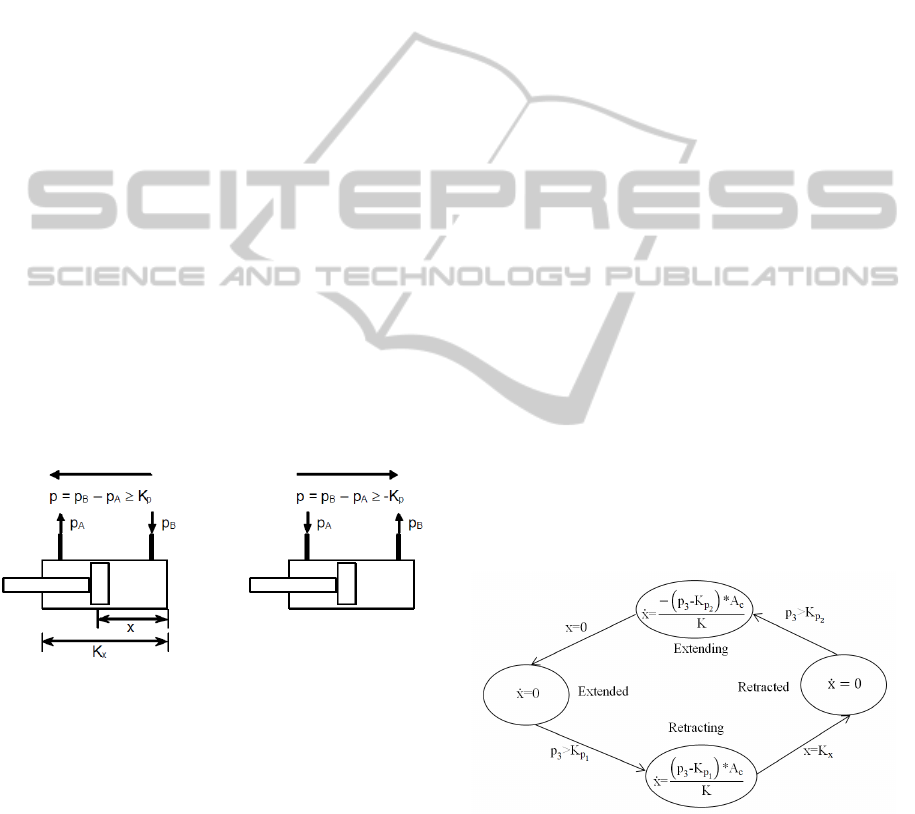
The architecture of the hydraulic part is described in
Figure 3 and only the principles of the motion
mechanism are discussed. The landing gear motion
is performed by a set of actuating cylinders. The
cylinder piston position corresponds to the landing
gear position and for each landing gear, a cylinder
retracts or extends it. Hydraulic power is provided to
the cylinders by a set of electro-valves, where one
main electro-valve supplies the specific electro-
valves for closing or opening with hydraulic power
Modeling&SimulationFrameworkfortheInclusionofSimulationObjectivesbyAbstraction
389
from the aircraft hydraulic circuit. The hydraulic
power is supplied to the landing gear circuit by a
pump with flow Q. The actuator part of the model is
inspired from a MATLAB example of the single
hydraulic cylinder simulation (MATLAB, 2014).
The architecture of the actuator cylinder is same
except for the presence of two openings at the ends
of actuator cylinder marked A and B denoting
retracted and extended positions respectively.
The working mechanism is briefly given as
follows, initially the control logic receives the pilot
command to extend or retract and, activates the
pump. As the flow from pump is passed through the
opening main control valve orifice with area A
, the
pressure, p
3
starts building at the end A or B,
depending on the pilot input C
,to extend or C
, to
retract the gear. Once the pressure differential
exceeds a certain threshold, K
∨
, the piston starts
moving until it reaches the other end or chamber
pressure equalizes the pump pressure, whichever is
earlier. Modeling abstractions such as flow
coefficients (F
,F
&F
, leakage phenomenon,
orifice model are kept the same as described in the
example for the sake of simplicity. Similarly, the
dynamic effect of aerodynamic or ground reactions
is not considered and interaction with other aircraft
systems is also not considered.
Figure 4: Actuator model (Boniol, 2014).
The inertial differential pressure at the ends A and B
are K
and K
and the dwell time when pressure is
below these limits corresponds to the unlock time
from the current mode. The length of cylinder is
given by K
x
.
3.2 System Dynamics & Simulation
The SUT is modelled as a Finite State Machine
(FSM) abstraction, a data type state aggregation
abstraction with hypothesis being the system
dynamics has four different modes depending on the
pilot input and actuator response.
Retracted : The piston is at position A and the
differential pressure is below the threshold.
Extending : The modulus of differential pressure
is above the threshold, K
, and the piston starts
moving from A.
Extended : The piston is at position B
Retracting : The modulus of differential pressure
is above the threshold, K
, and the piston starts
moving from B.
The system remains at the retracted or extended
position indefinitely until pilot command has been
initiated or failure of hydraulic circuit or both.
The system is modeled in SIMULINK and
Stateflow, a widely used commercial tool in
modeling and simulation of complex reactive
systems based on the finite state machine described
by events and actions. Simulations are carried out
using a variable step ODE45 solver. Alternatively,
such a hybrid system could be modeled in DEVS
formalism and solved using QSS algorithms which
are more amenable to hybrid system simulation as
the state events can be handled much more
efficiently by state-quantization algorithms than by
time-slicing algorithms.
The SUT is the control logic with the
environmental models being that of actuator, pump
and main control valve. The generator given below
supplies the input to generate input segments, Ω
of
pump flow and main control valve profile apart from
pilot commands
The switching modes are illustrated in the
following figure.
Figure 5: Landing gear hybrid system.
3.3 Simulation Requirements
Broadly, the requirements are classified as normal
and failure modes and the requirements related to
normal mode gear function alone listed in (Boniol,
2014) are taken for validity assessment.
Landing Gear
Retracting
Landing Gear
Extending
SIMULTECH2014-4thInternationalConferenceonSimulationandModelingMethodologies,Technologiesand
Applications
390
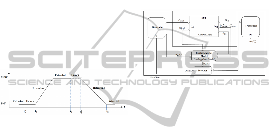
The high level SOU functional objective is
reaching the mode of operation for the given
command. The system should start from extended
mode and reach retracted mode when retract
command is given and vice versa for extend
command.
The other SOU is defined as the data class type
abstraction with validity criteria being error
tolerance on the maximum time of extending and
retracting denoted by t
extend
and t
retract
respectively.
φ
≔∀C
1
|t
1
t
2
t
extend
∨
∀C
2
|t
t
t
retrac
t
(19)
where, t
1
is the unlock time (when p
3
<K
), t
2
is the
time of extension, t
is the unlock time (when
p
3
<K
) and t
is the time of retraction. The
simulation requirement given in the form of
temporal profile with gear angle being measured
from horizontal plane is shown in figure 6.
Figure 6: Landing gear output requirement.
The state constraints are given as
∅
M
{p
3
∈0p
lim
} ∪{x∈0K
x
}
(20)
The simulation is valid if it satisfies the functional
and temporal requirements without violating
constraints.
3.4 Experimental Frame
The specification of the experimental frame defined
in Eq 1 is given as follows.
T =
The input and output of the EF are
I
E
={start/stop
O
E
=
ϴ
The input and output of the SUT are
I
M
=Y
G→M
⋃Y
EM→M
{x,p
3
,C
1
,C
2
O
M
=Y
M→G
⋃Y
M→EM
A
extend
m
,A
retract
n
,S
i
where
i→d gives the interconnection relation
m,n
= (A,B)∨(B,A)is the retracting or extending
valves
id = {retracted, retracting, extended, extending} are
the states describing the phase of the simulation.
The input segments of the EF and model are given
based on Eq 1. The acceptor segments are given by
Ω
C
S
id
,t
,(Y
M→EM
,t)
(21)
The environmental abstractions are assumed to be
ideal with respect to simulation requirements and
only the primary EF components abstractions are
discussed in the following section.
The experimental frame is illustrated in figure 7.
Figure 7: Landing gear hybrid system.
The interconnection between EF and model
components can be seen and such a definition helps
in coherent model development with respect to
simulation objectives.
3.4.1 Primary EF Abstractions
The generator, acceptor and transducer are described
below.
Generator, G: The input stimulii are the pilot
command to retract or extend the gear, pump flow
parameters of the main control valve orifice area and
pump flow profile.
M
G
=< T, X
G
,Y
G
>
(22)
where,X
G
=I
E
,
Y
G
={{Q,C
Ai
,C
}|cmd={retract, extend}}
C
Ai
is the main orifice valve opening profile.
The computation class abstraction is employed in
the form of a Look Up Table and linear interpolation
between data points d for the pump flow and valve
opening profile. The pilot command is abstracted as
a simple flag.
α
G
1
M
G
C
≔ f
(t,d)
(23)
M
G
C
is the concrete system specification of pump and
main control valve. f
is the linear map between data
points and time. The design abstraction, α
G
d
defined
in section 2.3, in this case is Q and C
Ai
.
Modeling&SimulationFrameworkfortheInclusionofSimulationObjectivesbyAbstraction
391

Transducer, T: The state of the model is
transduced in terms of gear rotation angle. The
transducer model is given by
M
T
=<T,X
T
,Y
T
>
(24)
where, X
T
={S
id
} Y
T
={ϴ|O
E
}
The transducer is abstracted as
Y
T
=
0 if S
id
=S
retract
f(x) if S
id
=(S
retracting
∨S
extending
)
90 if S
id
=S
extend
(25)
The map could be a simple linear function (eg:
90*(K
x
/x)) or may be dependent on velocity,
transmission delay etc.
Acceptor, A : The acceptor includes conditions
to check physical violation constraints such as
negative pressure defined as ∅
M
and semantics of
modes formalized in temporal logic.
α
1
M
C
≔
C
∧S
retracted
→◊S
extended
∨
C
∧S
extended
→◊S
retracted
(26)
where M
A
C
is the concrete acceptance conditions
specified in temporal logic formalism. Simulation
validity conditions could also be specified in it.
3.4.2 Results
A typical retract and extend operation of the landing
gear is shown below for a sample simulation
Figure 8: Landing gear output.
The fall in pressure at the pump, p
1
and subsequent
rise in pressure at the main control valve, p
2
and
downstream in the chamber, p
3
are seen. The piston
displacement, x for both extending (red) and
retracting (green) until it reaches other end of
cylinder is seen. In failure cases such as pump
failure, the piston stops before it reaches the other
end, which is not shown here. In essence, in normal
mode, once the piston reaches the other end, the
control logic closes the control valve and pressure
equalises in the circuit. For the sake of simplicity the
closing of main valve is not simulated.
The method allows to abstract the valid primary
EF components with respect to requirements based
on sample simulation runs. In the present simulation
the pump flow, Q and main valve opening, A
are
the input design parameters, I
M
d
. Recalling definition
in section 2.3, the generator design abstraction,
α
G
d
∈α
G
resulting in model input, Ω
M
d
∈Ω
M
driving
the simulation output is given by notation, α
G
d
↦
Ω
M
d
. Then the trace inclusion criteria allows to
classify them as
Valid :
α
G
d
↦Ω
M
d
|⊨φ
1
∧x,p
3
∈∅
M
Invalid:
α
G
d
↦Ω
M
d
|⊭φ
1
∧x,p
3
∈∅
M
Partially Valid:
α
G
d
↦Ω
M
d1
∈Ω
M
d
|⊨φ
1
∧x,p
3
∈∅
M
α
G
d
↦Ω
M
d2
∈Ω
M
d
|⊭φ
1
∧x,p
3
∈∅
M
Incompatible:
α
G
d
↦Ω
M
d
|⊭x,p
3
∈∅
M
(27)
The pump flow and cross section parameters of main
valve are thus classified with respect to simulation
objectives. Similar such abstraction for transducer
α
T
d
∈α
T
and acceptor α
A
d
∈α
A
driving the SUT can
be defined respectively, though it is not used in the
current study. Such design abstractions can help for
example drive the simulation to its objective by
observing and monitoring the results. The aggregate
effects of all such primary abstractions are observed
onto the model output.
It may be noted that the requirements φ
defined
belong to temporal class in that in certain cases
validation of a lower level requirement implicitly
validates the higher level requirement. Assuming the
acceptor abstraction α
1
is given as a requirement φ
then validation of temporal behaviour specified as
φ
implies validation of semantics of mode specified
as φ
.
The abstraction influence of primary EF
components on simulation validity can thus be
studied using such a validity criteria. Abstraction
classification and hierarchical composition
implemented in a tool will help in extracting
abstractions which are necessary and consistent with
simulation objectives. Building a repository of such
abstractions with respect to objectives could be used
0 0.01 0.02 0.03 0.04 0.05 0.06 0.07 0.08 0.09 0.1
0
0.5
1
1.5
2
x 10
6
Pressure (P a)
Pr e ssu r e
0 0.01 0.02 0.03 0.04 0.05 0.06 0.07 0.08 0.09 0.1
-0.01
0
0.01
0.02
0.03
Time (s)
Displacem ent (m )
Displacem ent
p1
p2
p3
Extending displace ment
Kx
Retracting displacement
SIMULTECH2014-4thInternationalConferenceonSimulationandModelingMethodologies,Technologiesand
Applications
392

to derive and reuse concepts based on the ontology
framework, also based on the lattice concepts. The
unified simulation method thus helps in better
development of models corresponding to
requirements.
4 FUTURE WORK
The present study deals with primary EF component
abstraction compatibility with SOU. The notions are
based on trace inclusion and a formal tool needs to
be built to quantify this abstraction. However, notion
of reachability is more pertinent than simulation for
hybrid systems since an exhaustive breadth first
search of state space through reachability analysis,
difficult as it might be in terms of computational
cost, yields formal verification of system. In this
regard, various reachability tools such as MATISSE,
UPPAAL, StateEx may be used and the inclusion
relation of reachable state space of SDU with respect
to SOU could be checked. Problems of scalability of
these reachability methods were discussed widely in
literature with potential solutions of using
abstractions to alleviate the computational burden.
The next step would be extending this method of
reachability inclusion through formal verification
tools.
The influence of modeling abstractions
especially of environmental models in EF are not
discussed here and quantification of abstraction
effect on the model reachability with respect to its
objective is of fundamental importance in the usage
of simulation as a means of analysis and design of
real world systems. A correct ‘by design’ of
abstraction with respect to simulation objectives
based on the concepts of approximate bisimulation
[Girard, 2007] and Galois connections [Cousot,
1992] is being studied. Such a holistic approach in
considering the objectives of simulation explicitly
into modeling via abstractions will help address the
problem of validity and fidelity in simulation.
5 CONCLUSIONS
Primary EF component abstraction in input stimuli
has been explained with respect to simulation
objectives. The hierarchical abstraction for class of
abstraction is explained with its correspondence to
simulation objective. Validity is assessed with a
behavioural compatibility criteria based on trace
inclusion. The method implemented here is not
correct by design but rather employed in classical
iterative fashion which is clearly neither optimal nor
formal in its approach. A rigorous mathematical
framework in synthesising such an abstraction with
respect to simulation objective would be the next
step. However, the current study lays sufficient
ground work in terms of assessment methodology
for a formal abstraction compatibility criterion to be
developed.
ACKNOWLEDGEMENTS
The authors would like to thank Richard Johnson
and Bernard Mattos for reviewing the paper and
Damien Foures for fruitful discussions on the
landing gear example.
REFERENCES
Albert, Vincent, 2009, Simulation validity assessment in
the context of embedded system design, Phd Thesis,
LAAS-CNRS, University of Toulouse, Unpublished.
Albert, V, Nketsa, A, Seguin, C, 2010, Verifying trace
inclusion between an experimental frame and a model,
DEVS Integrative Modeling and Simulation
Symposium.
Boniol, F, Wiels, V, 2014, The Landing Gear Case Study,
4
th
International ABZ Conference, Case study track.
Cousot, Patrick, 1992, Abstract Interpretation
Frameworks, Journal of Logic and Computation,
volume 2, pages 511-547.
Foures, D, Albert, V, Nkesta, A, 2013, Simulation
validation using the compatibility between simulation
model and experimental frame, Proceedings of the
2013 Summer Computer Simulation Conference,
Society for Modeling & Simulation International,
Vista, CA, Article 55 , 7 pages.
Foures, D, Albert, V, Nkesta, A, 2012, Formal
compatibility of experimental frame concept and FD-
DEVS model, 9th International Conference on
Modeling, Optimization & Simulation, Bordeaux,
France.
Girard, A, Pappas, G J, 2007, Approximation Metrics for
Discrete and Continuous Systems, IEEE Transactions
on Automatic Control, Volume 52, Issue 5, pages 782-
798.
Man-Kit-Leung, J, Mandl, T, Lee, E A, Latronico, E,
Shelton, C, Tripakis, S, Lickly, B, 2009, Scalable
semantic annotation using lattice based ontologies.
Lecture Notes in Computer Science, Volume 5795, pp
393-407.
MATLAB SIMULINK Single hydraulic cylinder
simulation, SIMULINK R2014a Example,
http://www.mathworks.fr/fr/help/simulink/examples/si
ngle-hydraulic-cylinder-simulation.html.
Modeling&SimulationFrameworkfortheInclusionofSimulationObjectivesbyAbstraction
393

Traoré, M K, Muzzy, A, 2006, Capturing the dual
relationship between simulation models and their
context, Simulation Modelling Practice and Theory
14(2): 126–142.
Zeigler, B P, 1984, Theory of Modelling and Simulation,
Krieger Publishing Co., Inc., Melbourne, FL, USA.
SIMULTECH2014-4thInternationalConferenceonSimulationandModelingMethodologies,Technologiesand
Applications
394
