Soil Strength-based Estimation of Optimal Control Parameters
for Wheeled Robots on Rough Terrain
Jayoung Kim and Jihong Lee
Dept. Of Mechatronics Engineering, Chungnam National University, Gungdong, Daejeon, Korea
Keywords: Optimal Control Parameter, Maximum Traction Coefficient, Optimal Slip Ratio, Tractive Efficiency, Soil
Strength, Vehicle Dynamics, State Observer, Soil Identification, Wheeled Robot, Rough Terrain.
Abstract: On rough terrain, there are a variety of soil types having different soil strength. It means that it is needed for
outdoor robots to change wheel control strategies since optimal slip and maximum traction levels on wheels
differ depending on soil strength. Therefore this paper proposes an algorithm for acquiring optimal control
parameters, such as maximum traction coefficient and optimal slip ratio to maximize traction or minimize
energy consumption, based on estimating strength of soils. In this paper the optimal models of wheel
traction and slip are derived through indoor experiments by a testbed for analysis of wheel-terrain
interactions on three types of soil; grass, gravel and sand. For estimating soil strength, actual traction
coefficient, including information of motion resistance, is observed by a state estimator related to wheeled
robot dynamics. The actual traction coefficient and slip ratio on wheels are employed to estimate soil
strength by a numerical method on the basis of derived optimal models. The proposed algorithm was
verified through real driving experiments of a wheeled robot on various types of soil.
1 INTRODUCTION
Outdoor wheeled robots have overcame obstructions
of moving on rough terrains, such as a slippery
surface or a steep slope, in order to fulfil important
tasks regarding the purpose of exploration,
reconnaissance, rescue, etc. For achieving such goals,
wheeled robots should have abilities to handle two
kinds of characteristic changes on rough terrains; a
change of soil types (slippery or non-slippery) and
surface shapes (flat or steep). Both the terrain
characteristic changes are crucial factors in the
decision regarding optimal wheel slip or traction as a
control parameter of a wheel controller since tractive
force of a wheel is differently exerted on a surface
according to such changes (Terry et al., 2008, Krebs
et al., 2010, Joo et al., 2013, Ding et al, 2010,
Ishigami et al., 2008, Brooks et al., 2012). In case of
changing surface shapes, it is relatively easy for
wheeled robots to realize the level of the change by
motion sensors like inertial measurement units
(IMU). On the contrary to this, it is not such an easy
undertaking to judge a type of soil where a robot is
operated in spite of using various sensors mounted
on a robot. To solve this issue, many researches
related to soil identification have been introduced in
the field of robotics.
The studies on soil identification based on
proprioceptive sensor data, not including dynamic
state information of a moving robot, have been
proposed. As proprioceptive sensors, the vibration
information of an accelerometer or IMU and the
current information of wheel motors were used to
make the data signals, which are transformed into
soil feature data in frequency domain using a Fast
Fourier Transform (FFT). The soil feature data were
classified into one of pre-learned soil models by a
support vector machine (SVM) (Brooks et al., 2012,
Iagnemma et al., 2005) or a probabilistic neural
network (PNN) (Coyle et al., 2008, Ojeda et al.,
2006). The performance of identifying a soil type
was verified through driving simulations or real
driving experiments on rough terrains. However,
these algorithms have physical limitations on real
applications of wheeled robots. First of all, the
vibration and current information is strongly
influenced by a robot speed and also a surface shape.
Therefore, although two robots move on the same
type of soil, it might indicate the result of identifying
one into another soil type depending on a robot
speed and a surface shape.
65
Kim J. and Lee J..
Soil Strength-based Estimation of Optimal Control Parameters for Wheeled Robots on Rough Terrain.
DOI: 10.5220/0005034900650073
In Proceedings of the 11th International Conference on Informatics in Control, Automation and Robotics (ICINCO-2014), pages 65-73
ISBN: 978-989-758-040-6
Copyright
c
 2014 SCITEPRESS (Science and Technology Publications, Lda.)

With wheel-soil interaction models for planetary
rovers on loose soils, the algorithms for soil
identification and for optimal wheel control were
proposed. In Brooks et al., 2012, the purpose of soil
identification is to estimate the maximum traction
through optimization of a traction force model,
based on observed rover wheel torque and sinkage.
And in Iagnemma et al., 2004, the purpose of soil
identification is to estimate key soil parameters,
cohesion c and internal friction angle ϕ which can be
used to compute maximum shear stress related to
maximum traction of wheels. To identify distinct
type of soil, in these researches, proprioceptive
sensor data are needed to be measured or estimated,
such as the vertical load, torque, wheel angular
speed, wheel linear speed and sinkage. The
algorithms were demonstrated using experimental
data from a four-wheeled robot in an outdoor Mars-
analogue environment. However, these methods
cannot be utilized for some wheeled robots like
military vehicles which are sometimes operated on
hard surfaces such as grass or firm soil, where the
sinkage does not occur because the force equations
become zero. On loose soils, it is also not easy to be
employed since it is difficult to precisely estimate
sinkage by vision or distance sensors.
To solve these problems, this paper proposes an
algorithm to estimate optimal control parameters;
maximum traction coefficient and optimal slip ratio
on rough surfaces with various soil types from a
hard surface through a loose surface, based on soil
strength without estimating wheel sinkage.
2 MODELLING OF OPTIMAL
CONTROL PARAMETERS
2.1 Improved Brixius Equation based
on Soil Strength
Brixius equation is well-known as one of empirical
methods, which express tractive characteristics of
bias-ply pneumatic tyres on a variety of soil types in
outdoor environments (Brixius, 1987, Tiwari et al.,
2010). To meet the purpose of this paper, previous
Brixius equation is changed into a function of wheel
slip ratio S and soil strength K which can be
measured or estimated by on-board sensors in real-
time, as shown in (3) – (6). In (1), slip ratio is a key
state variable and it is expressed as a function of the
linear velocity V
x
[m/s] and the circumference
velocity ωR
w
[m/s].
),max(
wx
xw
RV
VR
S




(1)
where R
w
[m] is the wheel radius and ω [rad/s] is the
wheel angular velocity. Soil strength K is also a
crucial variable for soil identification. Soil strength
K is actually estimated on a real-time system of a
robot by an algorithm for soil identification in this
paper.
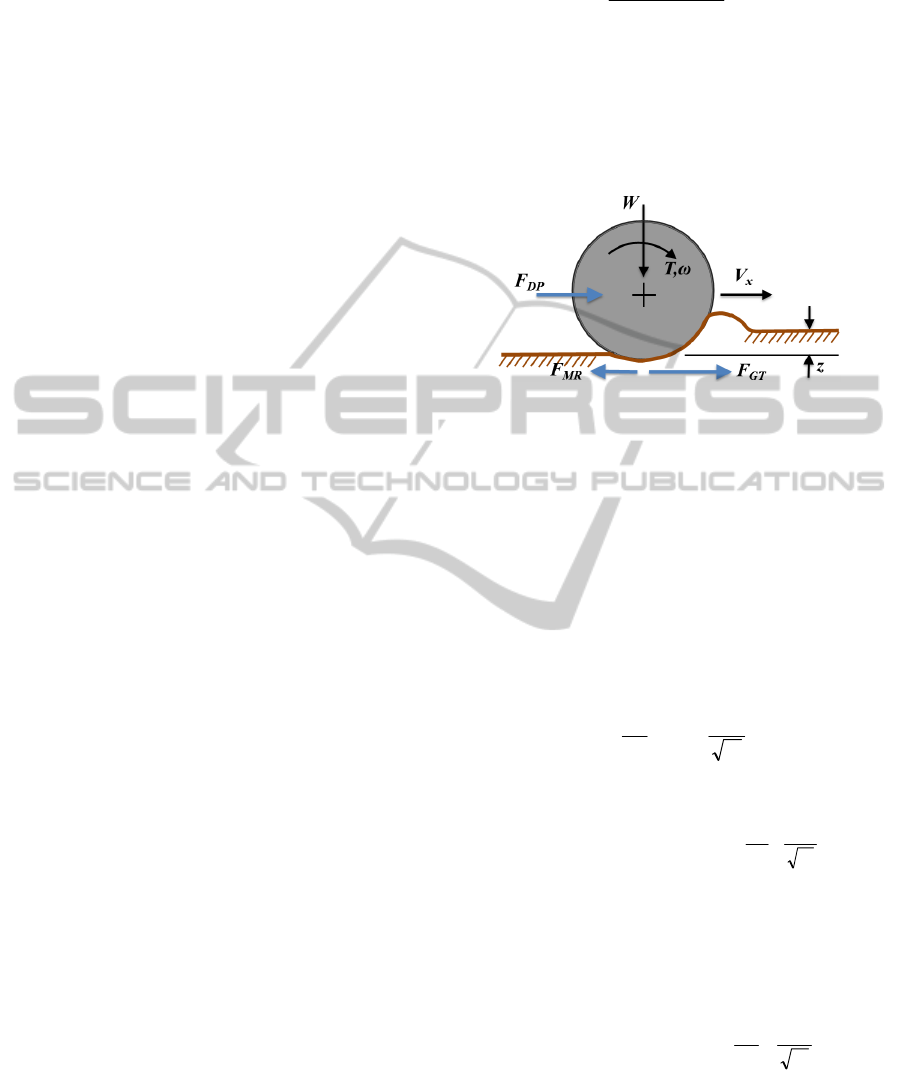
Figure 1: Forces acting on a driving wheel.
Figure 1 shows forces acting on a driving wheel during a
wheel-terrain interaction by wheel torque T [Nm] and
normal load W [N]. In (2), drawbar pull F
DP
[N] is
expressed by difference of gross traction F
GT
[N] and
motion resistance F
MR
[N].
MRGTDP
FFF 
(2)
By Brixius equation, gross traction F
GT
and motion
resistance F
MR
are as follows:


41
)1)(1(
3
2
CeeCWF
SC
KC
GT



(3)






 )(
6
4
5
K
SC
C
K
C
WF
MR
(4)
By (2), drawbar force F
DP
is defined as:








)()1)(1(
65
1
3
2
K
SC
K
C
eeCWF
SC
KC
DP

(5)
where
1
C
,
2
C
,
3
C
,
4
C
,
5
C
, and
6
C
are Brixius
constants and the values are determined by a
nonlinear regression technique. Equation (5) is
divided by normal load W as follows: (upper sign: S >
0, lower sign: S < 0)








)()1)(1(
65
1
3
2
K
SC
K
C
eeC
SC
KC


(6)
Equation (6) represents traction – slip curves
according to strength of soil K.
2.2 Derivation of OCP Models
For derivation of optimal slip models, indoor
ICINCO2014-11thInternationalConferenceonInformaticsinControl,AutomationandRobotics
66

experiments to acquire force data (F
DP
, F
GR
, and F
MR
)
in Figure 1 were conducted on three types of soil:
sand, gravel and grass where soil strengths are
different, as shown in Figure 2. In the system of the
testbed, the maximum angular velocity is 4.5 rad/s
and the maximum linear velocity is 32 cm/s.
Experimental slip conditions were controlled at 0.1,
0.2, 0.3, 0.4, 0.5 and 0.6. From measured data of the
testbed, Brixius equation can be completed based on
soil strength K of each soil type. Brixius constants in
the equations are calculated by a nonlinear
regression technique using a statistics program,
SPSS as follows: C
1
=1.3, C
2
=0.01, C
3
=7.058,
C
4
=0.04, C
5
=-5, C
6
=4. Strength of soils K are also
given: 50 (sand), 80 (gravel) and 200 (grass),
respectively.
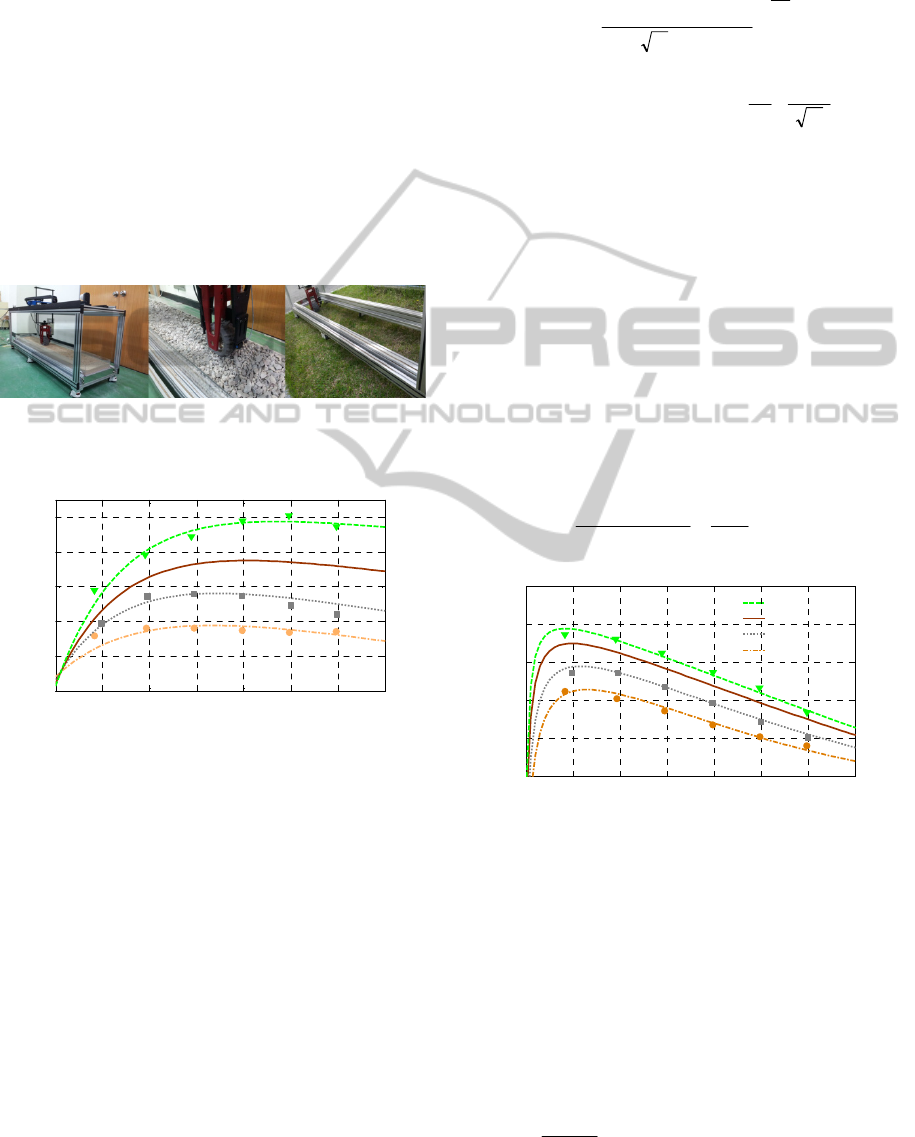
(a) Sand (b) Gravel (c) Grass
Figure 2: Wheel-soil interaction experiments using a testbed
on three types of soil.
Figure 3: Traction-slip curve on soil types; sand, gravel
and grass.
Using the given Brixius constants and soil strengths,
graphs of relation between wheel traction and slip
were drawn about the four types of soil from (6), as
shown in Figure 3. Actually, a curve in between
grass and gravel was not acquired from the indoor
experiments. When watching the gap between the
curves, it is possible to expect that there exists
another soil type which is harder than gravel or
softer than grass. The expected soil type (EST)
seems to have soil strength of K=120. On all the
curves, wheel traction is changed by increasing
wheel slip. And wheel traction indicates that it has
the maximum value at peak points on the curves
having a particular slip ratio. In this paper, the point
is named optimal slip ratio for maximum traction, S
T
.
And S
T
points can be calculated by partially
differentiating the traction-slip equation (6) with
respect to slip ratio S. Therefore the optimal slip
model for maximum traction and also the maximum
3
2
1
31
6
)1(
ln
C
KC
T
eKCC
C
S












(7)








)()1)(1(
65
1
3
2
K
SC
K
C
eeC
T
SC
KC
T
T


(8)
traction coefficient model are defined as functions of
soil strength K by (7) and (8), respectively.
In another case, Brixius equations can be
employed for analysis of wheel tractive efficiency of
(9). Equation (9) represents the degree of generated
drawbar pull F
DP
when gross traction F
GT
acts on
wheels. From Brixius equation (3) and (5), the
curves of tractive efficiency are described as shown
in Figure 4. All tractive efficiency on soil types
increases rapidly until reaching peak points near 0.1
of the slip ratio and decreases dramatically after that.
In this paper, the slip ratio is called optimal slip ratio
for TE, S
E
and it means that wheeled robots can
minimize energy consumption if the robots keep
wheel slip at S
E
while moving on rough terrains.
)1( S
F
F
powerInput
powerOutput
TE
GT
DP

(9)
Figure 4: Tractive efficiency on soil types; sand, gravel
and grass.
To derive an optimal slip model for maximum TE, it
is possible to partially differentiate the TE equation
(9) with respect to slip ratio S. However, there is
complexity for partial differentiation of (9) where
the nonlinear equation (3) and (5) are included. For
simplification, the S
E
model is derived as a linear
equation of soil strength K from real peak points on
each curve on the basis that the points of maximum
TE move on the curves at near 0.1 of slip ratios.
Derived S
E
model is as follows:


)(


K
S
E
,
9.5242,4.677 



(10)
0 0.1 0.2 0.3 0.4 0.5 0.6 0.7
0
0.2
0.4
0.6
0.8
1
Slip Ratio, S
Traction Coefficient, Mu
Grass ( K=200 )
Sand ( K=50 )
Expected Soil Type ( K=120 )
Gravel ( K=80 )
0 0.1 0.2 0.3 0.4 0.5 0.6 0.7
0
0.2
0.4
0.6
0.8
1
Slip Ratio, S
Tractive Efficiency, TE
Gravel ( K=80 )
Grass ( K=200 )
Sand ( K=50 )
EST ( K=120 )
SoilStrength-basedEstimationofOptimalControlParametersforWheeledRobotsonRoughTerrain
67

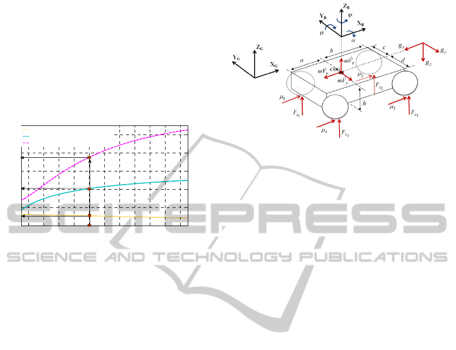
As an example, Figure 5 describes optimal values;
maximum traction coefficient μ
T
, optimal slip ratio for
traction S
T
and for TE S
E
calculated from the optimal
control parameter (OCP) models based on the soil strength
K=120. Derived OCP models include a wide range of soil
types from a hard surface like asphalt through a loose
surface like sand. Once soil strength K is estimated in the
range from zero to infinity, optimal control parameters are
determined and used to optimally adjust wheel rotations
according to the control purpose.
Figure 5: OCP curves depending on soil strength K.
3 PROPRIOCEPTIVE
ESTIMATION
OF SOIL STRENGTH
In this section, a method for estimation of soil
strength K was suggested. Soil strength K can be
simply determined through observing actual traction
coefficient μ and slip ratio S on the traction-slip
curve as shown in Figure 3. The estimator of the
actual traction coefficient is developed based on
wheeled robot dynamic models. Actual slip ratios of
wheels can be calculated by (1). Acquired real
information of the traction coefficient and the slip
ratio are employed to estimate soil strength K on the
traction-slip curve in Figure 3 by a numerical
method.
3.1 Estimation of Real Traction
Coefficient
The real traction coefficient estimator developed in
this paper, which does not cause a huge
computational burden or require derivations of
sensor signals, is based on a Kalman filter using
wheeled robot dynamics shown in Figure 6. The
motion equation of the robot on the X
R
-Y
R
-Z
R
robot
coordinates described in Figure 6 is
Rzxxxxz
MFFcFFdI
,
)()(
2143



(11)
Figure 6: Four-wheel drive, differentially steered robot.
where

is the yaw rate; I
z
represents the moment of
inertia of the robot, a and b are the distances from
the center of mass of the robot to the rear axle and
the front axle, respectively. And M
z,R
is the
resistance moment about Z
R
-axis and it is defined as:
)()(
3241
3
,
2
,
4
,
1
,, zRyzRyzRyzRyRz
FFbFFaM








(12)
where μ
y,R
is the lateral motion resistance coefficient
on Y
R
-axis and F
z
is the normal forces on wheels.
The subscript i
indicates that 1 is the left-rear wheel,
2 is the left-front wheel, 3 is the right-front wheel
and 4 is the right-rear wheel.
The motion equation for the wheel is as follows:
ii
Rxwxwii
FRFRTI
,






(13)
where T is the wheel torque, I
ω
is the moment of
inertial of a wheel, F
x
and F
x,R
are the longitudinal
traction and the motion resistance on X
R
-axis, which
can be obtained as follows:
ii
zix
FF


(14)
ii
z
i
RxRx
FF
,,


(15)
where μ is the longitudinal traction coefficient on
wheels and μ
x,R
is the motion resistance coefficient
on X
R
-axis. In (11)-(14), the normal force F
z
is
calculated by 3-dimentioanl normal force dynamics
defined as:
)()(
)()()(
432
camghmghmgcaVmhVmhVm
dcFdcbaFbaF
zyxzyx
zzz









(16)
)()(
)()()(
431
cbmghmghmgcbVmhVmhVm
dcbaFdcFbaF
zyxzyx
zzz








(17)
)()(
)()()(
421
dbmghmghmgdbVmhVmhVm
baFdcFdcbaF
zyxzyx
zzz









(18)
)()(
)()()(
321
damghmghmgdaVmhVmhVm
baFdcbaFdcF
zyxzyx
zzz









(19)
40 60 80 100 120 140 160 180 200 220 240
0
0.2
0.4
0.6
0.8
1
Soil Strength, K
S
E
, S
T
, Mu
T
Optimal Slip Ratio for Energy Efficiency
Optimal Slip Ratio for Maxmum Traction
Maximum Traction Coefficient
S
T
S
E
Mu
T
Mu
T
model
S
T
model
S
E
model
ICINCO2014-11thInternationalConferenceonInformaticsinControl,AutomationandRobotics
68

where m is the robot mass; h is the height from the
surface to the center of mass of the robot; c and d are
the distances from the center of mass of the robot to
the left wheels and the right wheels;
x
V

,
y
V

and
z
V

are the acceleration; g
x
, g
y
and g
z
are the gravity
force on the X
R
-Y
R
-Z
R
robot coordinates,
respectively. The gravity force is defined by (20)































































ccg
csg
sg
gcs
sc
cs
sc
g
g
g
G
G
G
G
TT
z
y
x
G
TT
R
0
0
0
010
0
0
0
001
GRRG
yx


where R
x
and R
y
are the rotation matrices about X
G
and Y
G
-axis, G
G
is the gravity force vector on the
global coordinate system. From (16)-(19), the
equations are transformed into a form of a matrix as
follows:
z
AFB 
(21)
where

T
zzzz
FFFF
4321

z
F
(22)

















0
0
0
0
badcbadc
badcdcba
dcbadcba
dcdcbaba
A
(23)



















)()(
)()(
)()(
)()(
damghmghmgdaVmhVmhVm
dbmghmghmgdbVmhVmhVm
cbmghmghmgc
bVmhVmhVm
camghmghmgcaVmhVmhVm
zyxzyx
zyxzyx
zyxzyx
zyxzyx




B
(24)
The normal forces are calculated by (25) defined as:
BAF
z
1

(25)
From (11)-(15), the states for the Kalman filter are
defined as follows:
T
y,Rx,R
][(t) ωψμμμx 
(26)
where
][
4321
μμμμμ
][
,
4321
x,Rx,Rx,Rx,RRx
μμμμμ
][
,
4321
y,Ry,Ry,Ry,RRy
μμμμμ
][
4321
ωωωωω
(27)
The measurements are

T
4321x
ωωωωψV

(t)z
(28)
where
)(
1
)(
1
4321
4321
4321 zzzz
xxxxx
FFFF
m
FFFF
m
V
 


(29)
Equations (11)-(15) and (26)-(29) are integrated to
build the following state-space system with process
noise w(t) and measurement noise v(t) as follows:
)()()()()( ttttt wBxAx 



)()()()( tttt vxHz


(33)
where A(t), B(t) and H(t) are defined in (30)-(32),
and their I
iⅹk
and O
iⅹk
denote an iⅹk identity matrix
and a zero matrix, respectively. Equation (33) is
discretized using zero-order hold for being
applicable to the discrete-time Kalman filter as
follows:
kkkkk
wBxAx 
1
kkkk
vxHz 
(34)
The algorithm of the discrete-time Kalman filter is
kkkk
BxAx 


ˆ
1
k
T
kkkk
WAPAM 
1
)(
ˆ
1
1 kkkk
T
kkkk
xHzVHPxx 


kkk
T
kkk
T
kkkk
MHVHMHHMMP
1
][


(35)
where W
k
and V
k
represent the covariance matrices
of w(t) and v(t). The estimator includes the motion
equations for the wheeled robot, but the traction
coefficients μ
i
are considered to be unknown
parameters to be estimated. And also, the
longitudinal motion resistance coefficients μ
x,Ri
are
included in the estimator in order to observe the
change of surface shapes and of soil types.
3.2 Estimation of Soil Strength
by Numerical Method
From derived actual traction coefficient and slip
ratio, soil strength K is simply estimated by a
numerical method. The numerical update rule of soil
strength K is defined as:
Enn
KK



1
(36)
where K
n+1
is the updated value of soil strength; K
n
is the previous value of soil strength, λ is the
learning rate selected in the range between 1 and 0,
η
E
is the learning weight defined as:
aa
e
a
ref
E
S
E
SS




(37)
SoilStrength-basedEstimationofOptimalControlParametersforWheeledRobotsonRoughTerrain
69

where μ
ref
is the reference value derived by the
estimator of real traction coefficient,
μ
e
is the
arbitrary value from (40) based on the traction-slip
curve in (6),
S
a
is the actual slip ratio of a robot and
E is the error model by (38). The reference value μ
ref
is integrated to consider actual tractive coefficient μ
with actual motion resistance μ
x,R
related to the
change of a surface shape and a soil type in (39).
The arbitrary value
μ
e
is calculated from the derived
traction-slip model by entering previous soil strength
K
n
and actual slip ratio S
a
as shown in (40). As initial
soil strength K
0
is selected as 250, the algorithm is
iteratively worked until the error
E becomes under
0.1.
eref
E




(38)
Rxref ,




(39)










)()1)(1(
65
1
32
n
a
n
SCKC
e
K
SC
K
C
eeC
an


(40)
4 EXPERIMENTAL
VERIFICATION IN OUTDOOR
ENVIRONMENTS
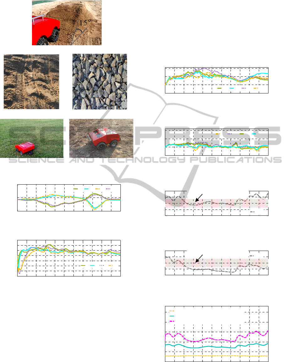
For verifying the proposed algorithm, a wheeled
robot was employed on five types of terrains; a
sandy slope (15 degrees), a rough sandy soil, a
gravel surface, a firm soil and a grassy surface as
shown in Figure 7. The robot size is 50cm long,
40cm wide and 30cm high. The weight of the robot
is 160N and it can move at max speed 2m/s. To
implement the proposed algorithm, it is most
important to estimate slip ratio between the linear
velocity of the robot and the circumference velocity
of the wheels. In this paper, additional wheel with
an encoder was used to measure the forward velocity
of the body. And the circumference velocity of the
wheels was acquired from the motor encoder of
wheels. Also, the 3-axis accelerations, the 3-axis
angles (roll, pitch and yaw) and angular rates on the
X
R
-Y
R
-Z
R
robot coordinates are measured by IMU.
At first, the performance of the suggested
algorithm was confirmed through the driving
experiment at robot speed 0.5 m/s on the sandy slope
in Figure 7 (a) containing the information of a
surface shape. Figure 8 shows estimated normal
forces of each wheel. The subscripts of
F
z
mean that
rf is the right-front wheel, rr is the right-rear wheel,
lr is the left-rear wheel and lf is the left-front wheel,
respectively.
In Figure 8, after 2 seconds, the robot is faced
with an uphill slope, and thereby the normal forces
on the front wheels decrease and the normal forces
on the rear wheels increase. And from about 7 to 10
seconds, the robot moves on a downhill sandy slope.
By the effect of the slope, the wheel slip data display
different tendencies on wheels each other. In Figure
9, from about 2 to 7 seconds, the front wheel slips
occur more than the rear wheel slips since the front
wheels lose the normal forces by the change of
surface shape. From Figure 8 and 9, it can be
confirmed how the changes of surface shapes
influence the robot dynamic states.
Figure 10 and 11 show the estimated traction
coefficients with or without compensating the
motion resistance regarding the surface shapes on
the sandy slope. Figure 10 represents values of a
combined model between the traction coefficient
μ
and the motion resistance coefficient μ
x,R
. Figure 11
indicates only the traction coefficient
μ. From the
results of the estimated actual traction coefficient























944444
5141
1712
4
3
214
3
21
)(
OII
OO
I
A

I
FR
I
FR
I
bF
I
bF
I
aF
I
aF
I
dF
I
dF
I
cF
I
cF
t
ii
zwzw
z
z
z
z
z
z
z
z
z
z
z
z
z
z
z
z
(30)
T
I
T
I
T
I
T
I
T
t









4
3
21
131
)( OB
(31)











55125
131
4
3
21
)(
IO
O
H
m
F
m
F
m
F
m
F
t
z
z
zz
(32)
ICINCO2014-11thInternationalConferenceonInformaticsinControl,AutomationandRobotics
70

(a) Sandy Slope (15°)
(b) Rough Sandy Soil (c) Gravel Surface
(d) Firm Soil (e) Grassy Surface
Figure 7: Experimental terrain types.
Figure 8: Estimated normal forces on the sandy slope.
Figure 9: Estimated slip ratios on the sandy slope.
and actual slip ratio, soil strength K on the sandy
slope was estimated by the numerical method as
shown in Figure 12 and 13. The convergence time
was average 0.01 seconds every samples. Figure 12
displays the flow of soil strength
K in the vicinity of
the desired area of soil strength of sand in contrast
with Figure 13. In Figure 13, the estimated soil
strength is gradually decreasing during the whole
time. From these results in Figure 12 and Figure 13,
it can be verified that the suggested algorithm
improves the performance of soil identification.
Figure 14 describes the results of estimating optimal
control parameters from the estimated soil strength
on the sandy slope. Actually, the pre-experimental
data were placed on about
K=50, μ
T
=0.4, S
T
=0.26
and
S
E
=0.12. In Figure 14, it is considered that the
outdoor experimental sandy surface had more
moisture, in that time, than the indoor experimental
sand surface though the estimated optimal control
parameters indicates slightly higher values than the
pre-experimental data.
Figure 10: Estimated traction coefficient μ with
compensating motion resistance on the sandy slope.
Figure 11: Estimated traction coefficient μ without
compensating motion resistance on the sandy slope.
Figure 12: Estimated soil strength K with compensating
motion resistance on the sandy slope.
Figure 13: Estimated soil strength K without compensating
motion resistance on the sandy slope.
Figure 14: Estimated optimal control parameters on the
sandy slope.
0 1 2 3 4 5 6 7 8 9 10 11
35
40
45
time [sec]
Normal Load, Fz [N]
Fz
rf
Fz
rr
Fz
lr
Fz
lf
0 1 2 3 4 5 6 7 8 9 10 11
-0.8
-0.6
-0.4
-0.2
0
0.2
0.4
time [sec]
Slip Ratio, S
S
rf
S
rr
S
lf
S
lr
0 1 2 3 4 5 6 7 8 9 10 11
-0.1
0
0.1
0.2
time [sec]
Mu
Mu
rf
Mu
rr
Mu
lf
Mu
lr
0 1 2 3 4 5 6 7 8 9 10 11
-0.1
0
0.1
0.2
time [sec]
Mu
Mu
lr
Mu
lf
Mu
rf
Mu
rr
0 1 2 3 4 5 6 7 8 9 10 11
20
40
60
80
100
time [sec]
Soil Strength, K
K
mean
0 1 2 3 4 5 6 7 8 9 10 11
20
40
60
80
100
time [sec]
Soil Strength, K
K
mean
0 1 2 3 4 5 6 7 8 9 10 11
0
0.2
0.4
0.6
0.8
1
S
E
, S
T
, Mu
T
time [sec]
(c) Optimal Slip Ratio for Energy Efficiency, S
E
(b) Optimal Slip Ratio for Maximum Traction, S
T
(a) Maximum Traction Coefficient, Mu
T
(b)
(c)
(a)
Desired Area
Desired Area
SoilStrength-basedEstimationofOptimalControlParametersforWheeledRobotsonRoughTerrain
71

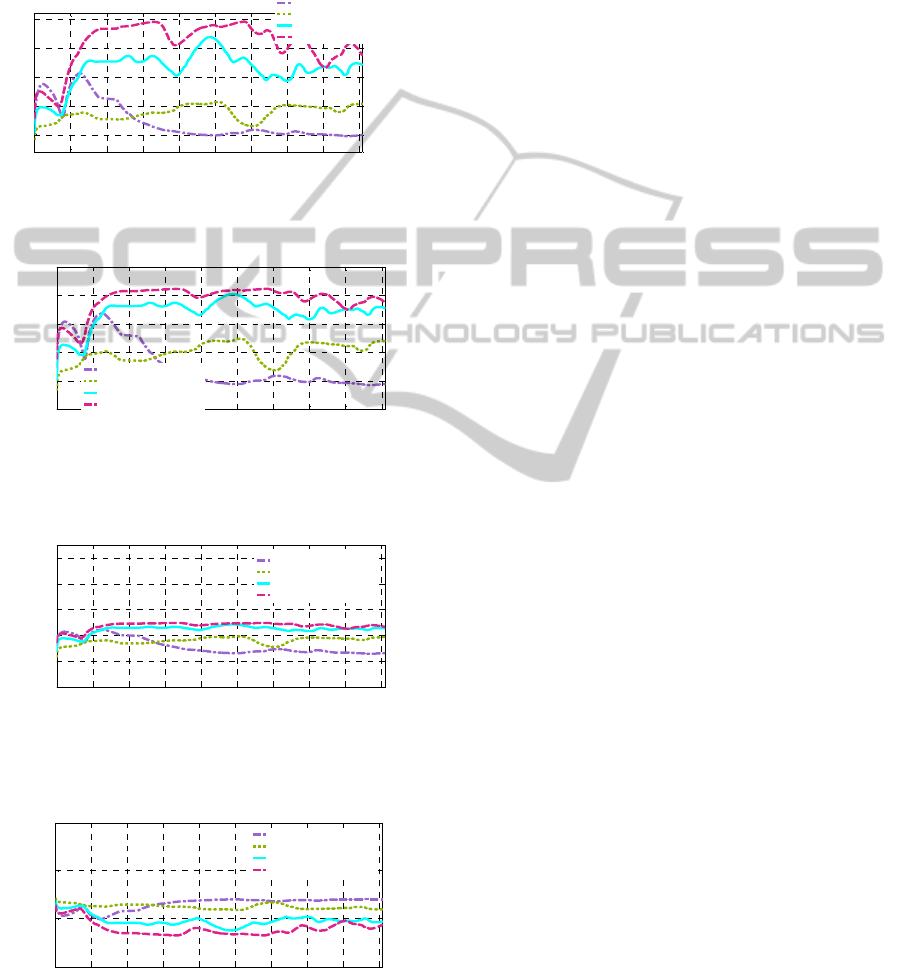
As other driving experiments at robot speed 1
m/s on the four types of soil in Figure 7 (b)–(e),
Figure 15 describes the results of estimating soil
strength
K depending on soil types. From 0 to 1
second, there are error values by the initial
measurement errors of wheel slip since the slip ratio
is very sensitive when the robot moves at low speed.
Figure 15: Estimated soil strength K on (a) firm soil (b)
grassy surface (c) gravel surface (d) rough sandy soil.
Figure 16: Estimated maximum traction coefficient μ
T
on
(a) firm soil (b) grassy surface (c) gravel surface (d) rough
sandy soil.
Figure 17: Estimated optimal slip ratio for traction S
T
on (a)
firm soil (b) grassy surface (c) gravel surface (d) rough
sandy soil.
Figure 18: Estimated optimal slip ratio for energy S
E
on (a)
firm soil (b) grassy surface (c) gravel surface (d) rough
sandy soil.
5 CONCLUSION
This paper proposed an algorithm for acquiring
optimal control parameters, such as maximum
traction coefficient and optimal slip ratio to
maximize traction or minimize energy consumption,
based on estimating strength of soils. In this paper
the optimal models for wheel traction and slip were
derived through indoor experiments using a testbed
for analysis of wheel-terrain interactions on three
types of soil; grass, gravel and sand. For estimating
soil strength, actual traction coefficient, including
information of motion resistance, was observed by
the DKF-based state estimator related to wheeled
robot dynamics. The actual traction coefficient and
slip ratio on wheels were employed to estimate soil
strength by the numerical method on the basis on
derived optimal models. The proposed algorithm
was verified through real driving experiments of the
wheeled robot on various types of soil. From the
evaluation of the estimation results, it could confirm
that the suggested algorithm has enough
performance to identify soil types on rough terrains.
ACKNOWLEDGEMENTS
The Authors gratefully acknowledge the support
from UTRC (Unmanned Technology Research
Center) at KAIST (Korea Advanced Institute of
Science and Technology), originally funded by
DAPA, ADD
REFERENCES
Jared D. Terry and Mark A. Minor, 2008, Traction
Estimation and Control for Mobile Robots using the
Wheel Slip Velocity, IEEE/RSJ International
Conference on Intelligent Robots and Systems.
Ambroise Krebs, Fabian Risch, Thomas Thueer, Jerome
Maye, Cedric Pradalier and Roland Siegwart, 2010,
Rover control based on an optimal torque distribution
– Application to 6 motorized wheels passive rover,
IEEE/RSJ International Conference on Intelligent
Robots and Systems.
Sang Hyun Joo, Jeong Han Lee, Yong Woon Park, Wand
Suk Yoo and Jihong Lee, 2013, Real time
traversability analysis to enhance rough terrain
navigation for an 6x6 autonomous vehicle, Journal of
Mechanical Science and Technology, Vol. 4, No. 27,
pp. 1125-1134.
Liang Ding, Haibo Gao, Zongquan Deng and Zhen Liu,
2010, Slip-Ratio-Coordinated Control of Planetary
Exploration Robots Traversing over Deformable
0 1 2 3 4 5 6 7 8 9
50
100
150
200
250
Soil Strength, K
time [sec]
On the rou
g
h sand
y
soil
On the gravel surface
On the grassy surface
On the firm soil
(a)
(b)
(c)
(d)
0 1 2 3 4 5 6 7 8 9
0.2
0.4
0.6
0.8
1
1.2
Maximum Traction Coefficient, M
u
time [sec]
On the rough sandy soil
On the gravel surface
On the grass surface
On the firm soil
(a)
(b)
(d)
(c)
0 1 2 3 4 5 6 7 8 9
0
0.2
0.4
0.6
0.8
1
Optimal Slip Ratio for Traction, S
T
time [sec]
On the rough sandy soil
On the gravel surface
On the grassy surface
On the firm soil
(d)
(c)
(a)
(b)
0 1 2 3 4 5 6 7 8 9
0.05
0.1
0.15
0.2
Optimal Slip Ratio for Energy, S
E
time [sec]
On the rough sandy soil
On the gravel surface
On the grassy surface
On the firm soil
(d)
(c)
(b)
(a)
ICINCO2014-11thInternationalConferenceonInformaticsinControl,AutomationandRobotics
72

Rough Terrain”, IEEE/RSJ International Conference
on Intelligent Robots and Systems.
Genya Ishigami, Keiji Nagatani and Kazuya Yoshida,
2008, Slope Traversal Experiments with Slip
Compensation Control for Lunar/Planetary
Exploration Rover, IEEE International Conference on
Robotics and Automation.
C. A Brooks and K. Iagnemma, 2012, Self-Supervised
Terrain Classification for Planetary Surface
Exploration Rovers, Journal of Field Robotics, vol. 29,
no. 1.
C. A Brooks and K. Iagnemma, 2005, Vibration-based
terrain classification for planetary exploration rovers,
IEEE Transactions on Robotics, 21(6), 1185–1191.
E. J. Coyle and E. G. Collins, 2008, Vibration-Based
Terrain Classification Using Surface Profile Input
Frequency Responses, IEEE International Conference
on Robotics and Automation.
L. Ojeda, J. Borenstein, G. Witus, and R. Karlsen, , 2006,
Terrain and Classification with a Mobile Robot,”
Journal of Field Characterization Robotics, vol. 23,
no. 2.
K. Iagnemma and S. Dubowsky, 2004, Mobile robots in
rough terrain: estimation, motion planning and control
with application to planetary rover,” Springer Tracts
in Advanced Robotics 12. Berlin: Springer.
W. W. Brixius, 1987, Traction prediction equations for
bias ply tires, ASAE, no. 87-1622.
V. K. Tiwari, K. P. Pandey, and P. K. Pranav, 2010, A
review on traction prediction equations, Journal of
Terramechanics, vol. 47, pp. 191-199.
SoilStrength-basedEstimationofOptimalControlParametersforWheeledRobotsonRoughTerrain
73