Active Vibration Control of a Super Element Model of a Thin-walled

Structure

Nader Ghareeb

and R¨udiger Schmidt

Department of Mechanical Engineering, Australian College of Kuwait, Kuwait City, Kuwait

Institute of General Mechanics, RWTH Aachen University of Technology, Aachen, Germany

Keywords:

Super Element, Lyapunov Stability Function Controller, Positive Position Feedback, Strain Rate Feedback.

Abstract:

Reducing vibration in ﬂexible structures has become a pivotal engineering problem and shifted the focus of

many research endeavors. One technique to achieve this target is to implement an active control system. A

conventional active control system is composed of a vibrating structure, a sensor to perceive the vibration,

an actuator to counteract the inﬂuence of disturbances causing vibration, and ﬁnally a controller to generate

the appropriate control signals. In this work, different linear controllers are used to attenuate the vibrations

of a cantilevered smart beam excited by its ﬁrst eigenmode. A ﬁnite element (FE) model of the smart beam

is initially created and then modiﬁed by using experimental data. The FE model is then reduced to a super

element (SE) model with a ﬁnite number of degrees of freedom (DOF). Controllers are applied directly to the

SE and the results are presented and compared.

1 INTRODUCTION

In modern engineering, weight optimization has a pri-

ority during the design of structures. However, opti-

mizing the weight results in lower stiffness and less

internal damping, causing the structure to become ex-

cessively prone to vibration. Vibration can lead to

additional noise, a decrease in stability, and even to

the failure of the structure itself (Ghareeb and Radov-

cic, 2009). To overcome this problem, active or smart

materials are implemented. The coupled electrome-

chanical properties of smart materials, which are il-

lustrated here in the form of piezoelectric ceram-

ics, make these smart materials well-suited for be-

ing used as distributed sensors and actuators for con-

troling structural response. Although the piezoelec-

tric effect was ﬁrst mentioned by Ha¨uy in 1817 and

demonstratedby Pierre and Jacques Curie in 1880, the

use of piezoelectric materials as actuators and sensors

for noise and vibration control has only been demon-

strated extensively over the past thirty years (Piefort,

2001). Bailey (Bailey, 1984) designed an active vibra-

tion damper for a cantilever beam using a distributed

parameter actuator consisting of a piezoelectric poly-

mer. Bailey and Hubbard (Bailey and Jr., 1985) de-

veloped and implemented three different control algo-

rithms to control the cantilevered beam vibration with

piezoactuators. Further, Crawley and de Luis (Craw-

ley and de Luis, 1987) and Crawley and Anderson

(Crawley and Anderson, 1990) presented a rigorous

study on the stress-strain-voltage behaviour of piezo-

electric elements bonded to beams. They observed

that the effective moments resulting from piezoactu-

ators can be regarded as concentrated at both ends of

the actuator while assuming a very thin bonding layer.

The practical implementation and use of the

piezoelectric actuators has been investigated in stud-

ies such as (Fanson and Chen, 1986) and (Moheimani

and Fleming, 2006). This work emphasizes the ca-

pabilities and applications of piezoelements as dis-

tributed vibration actuators and sensors by simulta-

neously controling a ﬁnite number of the inﬁnite set

of modes of the actual system. On the other hand,

the majority of investigations were carried out ei-

ther through experiments on the real model as in

(Waghulde et al., 2010),(Block and Strganan, 1998),

or by using 2D or 3D FE models of the smart struc-

ture as in (Varadan et al., 1996),(Allik and Hughes,

1970). However, in the FE work, the damping coefﬁ-

cients were not calculated but rather assumed, which

may not reﬂect the exact performance of the real

model.

The present work comprises the modeling and de-

sign of different active linear controllers to attenu-

ate the vibration of a cantilevered smart beam excited

by its ﬁrst eigenmode. The piezoactuator is initially

657

Ghareeb N. and Schmidt R..

Active Vibration Control of a Super Element Model of a Thin-walled Structure.

DOI: 10.5220/0005027206570664

In Proceedings of the 11th International Conference on Informatics in Control, Automation and Robotics (ICINCO-2014), pages 657-664

ISBN: 978-989-758-039-0

 2014 SCITEPRESS (Science and Technology Publications, Lda.)

modeled, and the relation between the voltage and the

moments at its ends is investigated. A modiﬁed FE

model of the smart beam based on ﬁrst-order shear de-

formation theory (FOSD) is then created. The damp-

ing coefﬁcients are calculated and added to the FE

model prior to the reduction to a SE model with a ﬁ-

nite number of DOF. The FE and SE models are

validated by performing a modal analysis and com-

paring the results with the experimental data. Finally,

two different control strategies are introduced and im-

plemented on the SE model of the smart beam: Posi-

tive position feedback (PPF), and strain rate feedback

(SRF). Results are then compared to the results of ap-

plying a Lyapunov stability function controller which

was developed in (Ghareeb and Schmidt, 2012). The

FE package SAMCEF is used for the creation of both

the FE and SE models, as well as for the implemen-

tation of the controllers in the SE model.

2 MODELING

The ﬁrst step in designing a control system is to

build a full representative mathematical model of

the real system including all the disturbances caus-

ing the unwanted vibration. The structural analytical

model can be derived either from physical laws (New-

ton’s motion laws, Lagrange’s equations of motion,

D’Alembert principle, etc), from test data using sys-

tem identiﬁcation methods (stochastic subspace iden-

tiﬁcation, prediction error method, etc), or by using

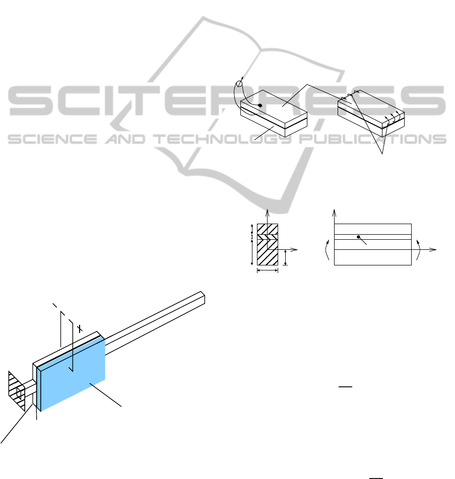
the FE method (Gawronski, 2004). The smart beam

used in this work consists of a steel beam, a bonding

layer and an actuator as seen in Figure 1.

actuator

beam

bonding layer

Figure 1: The smart beam.

2.1 Actuator Modeling

Using an actuator means imposing an appropriate

electric potential to control the vibration in the smart

structure (converse piezoelectric effect). Many FE

packages do not offer elements with electrical DOF.

On the other hand, the voltage applied by the actuator

can be represented by two equal moments with op-

posite directions concentrated at its ends (Fanson and

Chen, 1986). The relation between actuator moments

and voltage can be investigated, so that equivalent

moments are used instead as input to the controller

as illustrated in Figure 2. The structure is modeled as

one dimensional and the behavior of the piezoelectric

material is assumed to be linear throughout this work.

elastic material

−−>

piezoceramic material

equivalent moment pair Mp

Figure 2: The induced stresses from a piezoceramic actua-

tor.

actuator

adhesive

Mp Mp

beam

Figure 3: A schematic layout of the smart beam.

Considering the schematic layout of the middle

portion of the smart beam in Figure 3, if a voltage

V is applied accross the piezoelectric actuator while

assuming one dimensional deformation, the piezo-

electric strain ε

in the piezo is

· V (1)

with V as the voltage of the piezo-electric actuator,

the electric charge constant and t

the thickness

of the actuator.

Using Hooke’s law, the longitudinal stress is deﬁned

= E

· ε

= E

· V (2)

Where E

is the Young’s modulus of elasticity of the

piezoceramic actuator.

ICINCO2014-11thInternationalConferenceonInformaticsinControl,AutomationandRobotics

658

This stress generates a bending moment M

around

the neutral axis of the composite beam given by

−D)

· b· zdz (3)

and t

are the thickness values of the adhesive layer

and the beam, b is the width of the composite layer

at beam’s middle, and D the distance from beam’s

bottom to the neutral axis.

Considering equilibrium of moments about the

neutral axis gives

piezo

dA +

adhesive

dA +

beam

dA = 0

(4)

This means,

−D)

zdz + E

−D)

zdz +

−D)

(−D)

zdz = 0 (5)

is the thickness of the beam, E

the Young’s mod-

ulus of the adhesive and E

the Young’s modulus of

the steel beam.

D =

+ 2E

+ E

+ 2E

+ E

+ 2E

(6)

Substituting (6) and (2) in (3) determines the bending

moment generated by the piezo M

as a function of

the voltage V

) + E

+ 2t

)

+ E

d · b

·V

(7)

Since the relation between M

and V is now known,

the actuator moments will be taken instead of the volt-

age as the input to the controllers that are designed

and implementedin the next sections. The importance

of this achievement is that only mechanical DOF will

be included in the model.

2.2 FE Modeling of the Smart Beam

Many applications in structural dynamics can be suc-

cessful only when they are represented by an accurate

mathematical model. A way to derive this model is

to use FE modeling. In order to ﬁnd the best FE

model that represents the smart beam, the optimal

type and size of the ﬁnite elements must be selected.

For this reason, a modal analysis of the real beam is

indispensable. The modal analysis is experimentally

performed, and results of the natural frequencies are

compared with those from the FE model. A detailed

geometry of the smart beam is shown in Figure 4, and

the material properties and thickness of each part are

represented in Table 1.

layer

composite

10 75 130

Figure 4: A detailed geometry of the smart beam [dimen-

sions in mm].

Table 1: Parameters of the components of the smart beam.

Beam Bonding Actuator

Material steel epoxy PIC 151

Thickness [mm] 0.5 0.036 0.25

Density [kg/m

] 7900 1180 7800

Young’s mod. [MPa] 210000 3546 66667

The smart beam is created as a unique structure

but modeled as a composite shell with three layers

without any relative slip among their contact surfaces.

Furthermore, a composite shell element with eight

nodes based on the FOSD is used. To valiate the

FE model, a modal analysis is performed and the ﬁrst

two eigenfrequencies are read and compared to those

from the experiment. This is presented in Table 2. As

a boundary condition, the far left edge of the smart

beam is clamped.

Table 2: validation of element-type based on the modal

analysis.

FE model Experiment

eigenfreq. [Hz] 13.81 13.26

eigenfreq. [Hz] 42.67 41.14

2.2.1 Damping Characteristics

Damping parameters, which are of signiﬁcant impor-

tance in determining the dynamic response of struc-

tures, cannot be deduced deterministically from other

structural properties or even predicted by using the

FE technique. For simplicity and convenience the

damping is assumed to be viscous and frequency de-

pendent (Alipour and Zareian, 2008). This linear ap-

proach assumes that the damping matrix is a linear

combination of the mass and stiffness matrices. Al-

though this idea was suggested for mathematical con-

venience only, yet it allows the damping matrix to be

diagonalized simultaneously with the mass and stiff-

ness matrices, preserving the simplicity of uncoupled

real normal modes as in the undamped case (Adhikari

and Woodhouse, 2001).

ActiveVibrationControlofaSuperElementModelofaThin-walledStructure

659

The relation is

C = αM + β K (8)

where α and β are real scalars that need to be deter-

mined.

To ﬁnd out α and β , many methods can be ap-

plied like the method of Chowdhury and Dasgupta, or

the method of damping from normalised spectra (also

known as the half-power bandwidth method). These

methods and the way to ﬁnd the results hereafter are

explained in details in (Ghareeb, 2013). Both meth-

ods are used in this work and the results are depicted

in Table 3.

Table 3: Results of α and β using both methods.

Parameter Chowdhury Half-power

α 0.02577 0.02955

β 9.918× 10

−6

9.77× 10

−6

3 THE SUPER ELEMENT

TECHNIQUE

The main advantage of this technique (also called

substructure technique) is the ability to perform the

analysis of a complete structure by using the results

of prior analysis of different regions comprising the

whole structure. When a preliminary analysis of the

different parts is performed, the computation time and

the size of the whole system are reduced. However, all

DOF considered useless for the ﬁnal solution are con-

densed and the rest is retained. This means, the DOF

of the whole system will correspond to the retained

nodes plus a number of internal deformation modes,

(refer to SAMCEF tutorials). To construct a SE, or in

other words to remove the unwanted nodes and DOF

from the substructure, many methods are available.

In this work, The ”Component-mode method”, Also

known as Craig-Bampton method, is used (Craig and

Bampton, 1968).

3.1 SE Modeling

Before the SE is created, the retained nodes and the

condensed nodes must be designated and the num-

ber of internal modes to be used must be speciﬁed.

Once again, the number of modes must respond to

atleast ninety-ﬁve percent participation of the mass.

Based on the current work, ten internal modes are

used. The retained nodes are usually those where

boundary conditions are applied, or where stresses,

displacements, etc. are imposed or measured. On

these nodes the clamp is added and the actuators and

sensors are placed. All other nodes are considered as

condensed nodes. Concerning the smart beam used

in this work, there are ﬁve retained nodes in the SE

model (Figure 5) listed below:

• The SE is clamped at node 1

• The actuator moments, which will be the inputs to

the controller, are added at the nodes 2 and 3

• An additional sensor to measure the vibrations is

added at node 4 (to be used in future works)

• The sensor that measures the tip displacement is

located at node 5

1 4 5

2 3

Figure 5: The retained nodes of the SE.

3.2 Comparison between FE and SE

Model

In Table 4, a comparison between both models was

done. The number of elements, nodes, and DOF was

reduced and this has lead to a smaller structure and

thus less computation time.

Table 4: Comparison between FE and SE model.

FE model SE model

Number of nodes 8206 5

Number of elements 2575 1

DOF 49236 40

3.3 Validation of the SE Model

As shown in Table 5, results of modal analyses of

both models did not show a big difference concern-

ing the ﬁrst four eigenfrequencies. Since the excita-

tion is done only with the ﬁrst eigenfrequency, further

readings were not necessary. The SS representation is

then created upon specifying the type and position of

the inputs and outputs of the model.

Table 5: Comparison between the eigenfrequencies.

Eigenfreq. no. FE model SE model % Error

1 13.811 14.249 3.07

2 42.673 43.414 1.71

3 145.49 152.54 4.62

4 150.16 154.38 2.73

ICINCO2014-11thInternationalConferenceonInformaticsinControl,AutomationandRobotics

660

4 CONTROLLER DESIGN

The performance of smart structures for active vibra-

tion control depends strongly on the control algorithm

accompanied with it. In this part, the aim is to de-

sign some controllers capable of damping the vibra-

tion once the smart beam is excited by its ﬁrst eigen-

mode. After the excitation, the beam is left to vibrate

freely. Exactly at this moment, the controllers are ac-

tivated. Two vibration suppression methods are used

in this work: The positive position feedback control

(PPF) and the strain rate feedback control (SRF).

4.1 Positive Position Feedback

Control (PPF)

This method was ﬁrstly proposed by Goh and

Caughey for the collocated sensors and actuators

(Goh and Caughey, 1985). Later on, it was used by

Fanson and Caughey to control large space structures

(Fanson and Caughey, 1990). The basic concept of

the PPF is to feed the structural position coordinate

directly to the compensator and the product of the

compensator and a scaler gain positively back to the

structure.

The scalar equations governing the vibration of the

structure in a single mode and the PPF controller are

given as

ξ+ 2ζω

ξ+ ω

ξ = Gω

η (9)

η+ 2ζ

η+ ω

η = ω

ξ (10)

where ξ is the structural modal coordinate, η the com-

pensator modal coordinate, G the feedback gain, and

ζ and ζ

are the damping ratios, and ω and ω

the

natural frequencies of structure and compensator.

Since all the parts of the smart beam are integrated

in a single SE and the damping coefﬁcients for the

whole system are calculated and the ﬁrst eigenmode

of the model is excited, this means

= ζ (11)

= ω (12)

To validate this supposition, the structure motion at

the steady state for a single DOF system can have the

form

ξ(t) = αe

iωt

(13)

and the compensator will then respond as

η(t) = βe

i(ωt− φ)

(14)

where the phase angle φ and the magnitude β are

φ = tan

−1



2ζ

(ω/ω

)

1− (ω/ω

)



β =

[1− (ω/ω

)

]

+ [2ζ

(ω/ω

)]

Since the structure and compensator have same fre-

quency as it was assumed before, then

= 1

For this reason φ =

, and β =

2ζ

Substituting φ and β in (13) and (14), and then back-

substituting in (9) gives

ξ+ (2ζw+

2ζ

)

ξ+ w

ξ = 0 (15)

Comparing (15) to (9), it can be seen that with the

assumption of equal frequencies between the struc-

ture and the compensator, there is an increase in the

damping ratio, which is called active damping.

A Nyquist stability analysis of the system of scalar

equations (9) and (10) results in the necessary and suf-

ﬁcient condition for stability

stability if 0 < G < 1

Implementing the PPF controller in the smart struc-

ture used in this work, has damped the tip displace-

ment as can be seen in Figure 6.

20 22 24 26 28 30 32 34 36 38 40

−0.03

−0.02

−0.01

0.00

0.01

0.02

0.03

Time (s)

Tip displacement (m)

No control

PPF

Figure 6: Tip displacement vs. time with and without con-

trol.

In the FFT spectrum diagram which is shown

in Figure 7, the effect of the PPF controller on the

amplitude of the peak displacement of the smart

beam and its magnitude is illustrated.

4.2 Strain Rate Feedback Control (SRF)

The SRF control is used for active damping of a ﬂex-

ible space structure as in (Fei and Fang, 2006). With

this technique, the structural velocity coordinate is fed

back to the compensator while the compensator posi-

tion coordinate multiplied by a negative gain is fed

ActiveVibrationControlofaSuperElementModelofaThin-walledStructure

661

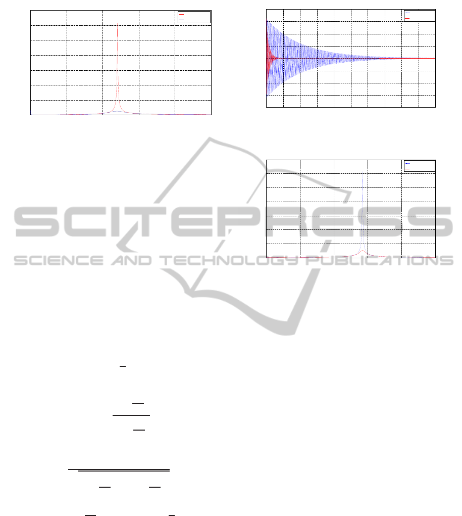
0 5 10 15 20 25

0.01

0.02

0.03

0.04

0.05

0.06

0.07

Frequency (Hz)

Amplitude (mm)

No control

PPF control

Figure 7: The FFT spectrum of the smart beam.

back to the structure. SRF has a wider active damp-

ing region and it can stabilize more than one mode if

given a sufﬁcient bandwidth.

The SRF model is presented as

ξ + 2ζ

ξ + ω

ξ = − Gω

η (16)

η + 2ζ

η + ω

η = ωc

ξ (17)

Similar to what has been done during the design of

the PPF controller, it’s also supposed that

ζ = ζ

(18)

= ω (19)

To validate this supposition, the structure motion at

the steady state for a single DOF system can have the

form

ξ(t) = αe

iωt

(20)

and the output of compesator at steady state will be

η = βe

i(ω+

− φ)

(21)

where

φ = tan

−1

2ζ

(

)

(1−

)

(22)

And magnitude β is given by

β =

(1−

)

+ (2ζ

)

(23)

When ω = ω

⇒

= 1, then ϕ =

⇒

ξ+ 2ζω

ξ+ (ω

+ Gβω

)ξ = 0 (24)

In this case, there will be an increase in the stiffness

of the structure (active stiffness). Moreover, the sta-

bility condition is not clearly deﬁned due to the fact

that the closed-loop damping and stiffness matrices of

the whole system cannot be symmetrized (Newman,

1992). The SRF controller has shown to be very ef-

fective in damping the ﬁrst eigenmode of the smart

beam. This is shwon in (Figure 8) and (Figure 9).

20 22 24 26 28 30 32 34 36 38 40

−0.04

−0.03

−0.02

−0.01

0.00

0.01

0.02

0.03

0.04

Time (s)

Tip displacement (m)

No control

SRF control

Figure 8: Tip displacement vs. time with and without con-

trol.

0 5 10 15 20 25

0.01

0.02

0.03

0.04

0.05

0.06

0.07

Frequency (Hz)

Amplitude (mm)

No control

SRF control

Figure 9: The FFT spectrum of the smart beam.

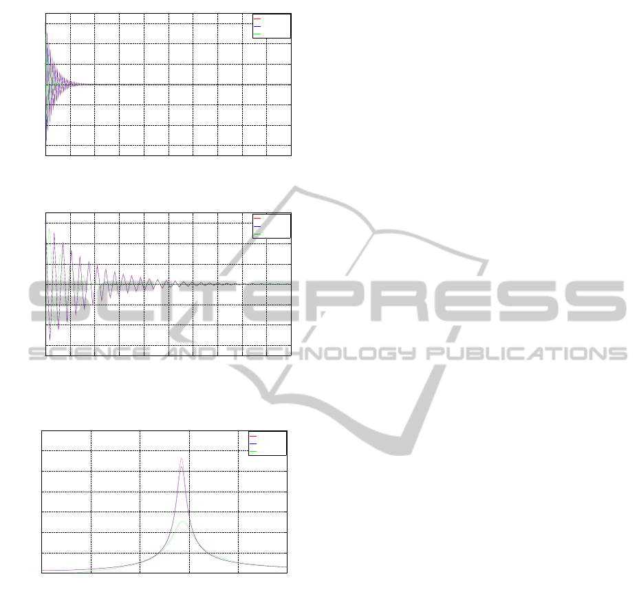
4.3 Comparison of Results of

Controllers

Comparing the results of the PPF and SRF con-

trollers, together with the Lyapunov stability control

strategy from (Ghareeb and Schmidt, 2012), some im-

portant facts were noticed. Firstly, the SE technique

has proved its efﬁciency by demanding low effort and

small computation time. Secondly, it was concluded

that the PPF controller needed much less time to sta-

bilize the system, in comparison to the other con-

trollers. This is shown in Figure 10 and Figure 11.

Thus, when the PPF controller was implemented,

it took about 0.8 seconds to stabilize the tip dis-

placement, while with other controllers it took about

2 seconds.

The SRF and Lyapunov control strategies pro-

duced similar results. This is due to the fact that in

both controllers, the velocity was the input parameter

to the system.

The effectiveness of the PPF is shown also in Fig-

ure 12 where the amplitude of the resonance of the

ﬁrst natural frequency is highly reduced in compari-

son to the other control strategies.

ICINCO2014-11thInternationalConferenceonInformaticsinControl,AutomationandRobotics

662

20 21 22 23 24 25 26 27 28 29 30

−0.03

−0.02

−0.01

0.00

0.01

0.02

0.03

Time (s)

Tip displacement (m)

Lyapunov

SRF

PPF

Figure 10: Tip displacement vs. time (SE model).

20 20.2 20.4 20.6 20.8 21 21.2 21.4 21.6 21.8 22

−0.03

−0.02

−0.01

0.00

0.01

0.02

0.03

Time (s)

Tip displacement (m)

Lyapunov

SRF

PPF

Figure 11: Tip displacement vs. time in a zoomed region of

Figure 10.

0 5 10 15 20 25

× 10

−3

Frequency (Hz)

Amplitude (mm)

Lyapunov

SRF

PPF

Figure 12: The FFT spectrum of the smart beam.

5 CONCLUSIONS

In this work, the basic procedures for the modeling

and simulation of a smart beam were presented. At

the beginning, the relation between actuator velocity

and actuator moment was derived. A FE model was

created and the damping coefﬁcients were calculated.

A SE model was then deduced from the FE model.

Different linear controllers were designed and imple-

mented on the SE to control the free body vibrations

of the cantilevered beam which was excited by its ﬁrst

eigenmode. The controllers proved to be very effec-

tive and the results were shown and compared. In the

future, other types of controllers will be designed and

implemented. Nevertheless, more eigenmodes will be

controlled and the possibility to implement the con-

trollers experimentally will be checked.

REFERENCES

Adhikari, S. and Woodhouse, J. (2001). Identiﬁcation of

damping: Part 1, viscous damping. Journal of Sound

and Vibration, 243, no.1:43–61.

Alipour, A. and Zareian, F. (2008). Study rayleigh damp-

ing in structures; uncertainties and treatments. In The

World Conference on Earthquake Engineering,

Beijing, China.

Allik, H. and Hughes, T. (1970). Finite element method

for piezoelectric vibration. International Journal for

Numerical Methods in Engineering, 2:151–157.

Bailey, T. (1984). Distributed-parameter vibration con-

trol of a cantilever beam using a distributed-parameter

actuator. Master’s thesis, Massachusetts Institute of

Technology.

Bailey, T. and Jr., J. H. (1985). Distributed piezoelectric-

polymer active vibration control of a cantilever beam.

AIAA Journal of Guidance and Control, 6, no.5:605–

611.

Block, J. and Strganan, T. (1998). Applied active control for

a nonlinear aeroelastic structure. Journal of Guidance,

Control, and Dynamics, 21, no.6:838–845.

Craig, R. and Bampton, M. (1968). Coupling of sub-

structures for dynamic analyses. AIAA Journal, 6,

no.7:1313–1319.

Crawley, E. and Anderson, E. (1990). Detailed models of

piezoceramic actuation of beams. Journal of Intelli-

gent Material Systems and Structures, 1, no.1:4–24.

Crawley, E. F. and de Luis, J. (1987). Use of piezoelectric

actuators as elements of intelligent structures. AIAA

Journal, 25, no.10:1373–1385.

Fanson, J. and Caughey, T. (1990). Positive position feed-

back control for large space structures. AIAA Journal,

28, no.4:717–724.

Fanson, J. and Chen, J. (1986). Structural control by the

use of piezoelectric active members. Proceedings

of NASA/DOD Control-Structures Interaction Confer-

ence, NASA CP-2447, 2:809–830.

Fei, J. and Fang, Y. (2006). Active feedback vibration sup-

pression of a ﬂexible steel cantilever beam using smart

materials. Proceedings of the First International Con-

ference on Innovative Computing, Information and

Control (ICICIC’06).

Gawronski, W. (2004). Advanced Structural Dynamics and

Active Control of Structures. Springer.

Ghareeb, N. (2013). Design and Implementation of Linear

Controllers for the Active Control of Reduced Models

of Thin-Walled Structures. PhD thesis, RWTH Aachen

University of Technology.

Ghareeb, N. and Radovcic, Y. (August 2009). Fatigue anal-

ysis of a wind turbine power train. DEWI magazin,

35:12–16.

ActiveVibrationControlofaSuperElementModelofaThin-walledStructure

663

Ghareeb, N. and Schmidt, R. (2012). Modeling and active

vibration control of a smart structure. In Proceedings

of the 9th International Conference on Informatics in

Control, Automation and Robotics (ICINCO 2012),

volume 1, pages 142–147, Rome.

Goh, C. and Caughey, T. (1985). On the stability problem

caused by ﬁnite actuator dynamics in the collocated

control of large space structures , 1985, vol. 41, no.

3, pp. 787-802. International Journal of Control, 41,

no.3:787–802.

Moheimani, S. and Fleming, A. (2006). Piezoelectric

Transducers for Vibration Control and Damping.

Springer.

Newman, S. (1992). Active damping control of a ﬂexible

space structure using piezoelectric sensors and actua-

tors. Master’s thesis, U.S. Naval Postgraduate School,

CA.

Piefort, V. (2001). Finite Element Modelling of Piezoelec-

tric Active Structures. PhD thesis, Universit Libre de

Bruxelles, Belgium.

Varadan, V., Lim, Y., and Varadan, V. (1996). Closed

loop ﬁnite-element modeling of active/passive damp-

ing in structural vibration control. Smart Materials

and Structures, 5, no.5:685–694.

Waghulde, K., Sinha, B., Patil, M., and Mishra, S. (2010).

Vibration control of cantilever smart beam by us-

ing piezoelectric actuators and sensors. International

Journal of Engineering and Technology, 2, no.4:259–

262.

ICINCO2014-11thInternationalConferenceonInformaticsinControl,AutomationandRobotics

664

REFERENCES

Adhikari, S. and Woodhouse, J. (2001). Identification of