Task Level Optimal Control of a Simulated Ball Batting Robot

Dennis Sch

uthe and Udo Frese

Multi-Sensor Interactive Systems Group, University of Bremen, Enrique-Schmidt-Str. 5, Bremen, Germany

Keywords:

Optimal Control, Finite Horizon, LQR, Afﬁne System, Entertainment Robot, Redundancy, Flexible Joints.

Abstract:

We developed a task-oriented controller based on optimal ﬁnite horizon control. We demonstrate this on a

ﬂexible ball playing robot with redundant degrees of freedom. The task is to reach a speciﬁed Cartesian po-

sition and velocity of the bat at a speciﬁed time, in order to rebound the ball. The controller must maintain

high accuracy and react to disturbances and changing conditions. Therefore, we formulate this as an optimal

control problem giving the controller the possibility to autonomously distribute motor torques amongst the re-

dundant degrees of freedom. In simulations, we show the accuracy of the controller, the intelligent distribution

of motor torques, as well as robustness against disturbances and adaptation to changing conditions.

1 INTRODUCTION

Targeted ball hitting poses a great challenge to the hu-

man bio-physical system. From perception of the ball

to the exact hitting-time many steps have to be pro-

cessed. Herein the “control” of muscles to trigger the

bat precisely to the predicted position with appropri-

ate speed has a crucial role in playing the ball back. In

performing this action, it would seem that the human

brain solves an optimal control problem. Our goal is

to achieve something similar on a ball playing enter-

tainment robot (Figure 1 ). Therefore, we developed

an optimal ﬁnite horizon controller handling the task

of being at a speciﬁed time in a speciﬁed position with

a speciﬁed velocity.

1.1 System

Our robot is a 2.1 m tall ball playing entertainment

robot called “Doggy”. It hits balls with its head,

which consists of a 40cm styrofoam sphere ﬁtted to a

carbon rod. The rod is attached to three revolute joints

having one common point where their rotational axes

intersect (Figure 2). The ﬁrst axis is acting like a hip,

giving the robot a redundant degree of freedom (DOF)

with the intention to make it more agile. Thus, the

end-effector (EOF) moves on a sphere (actually par-

tially due to joint limits) and we have three redundant

joints to control the 2 DOF. As the end-effector (bat)

is a sphere the orientation does not matter. Further-

more, our stereo camera is mounted after the ﬁrst axis

allowing it to turn and change the viewing direction.

Figure 1: The 2.1 m tall ball playing entertainment robot

“Doggy”.

The joints are driven by DC motors through tooth

belts, resulting in elasticity, which needs to be taken

into account by the controller.

1.2 Problem Statement

The problem is to be at a speciﬁed time T in a spec-

iﬁed position p with a speciﬁed velocity v with the

centre of the robots head to play back a thrown ball.

The cost of doing so should be brought to a minimum,

i. e. the reduction of the motors torque. Thus, the re-

Schüthe D. and Frese U..

Task Level Optimal Control of a Simulated Ball Batting Robot.

DOI: 10.5220/0005026100450056

In Proceedings of the 11th International Conference on Informatics in Control, Automation and Robotics (ICINCO-2014), pages 45-56

ISBN: 978-989-758-040-6

 2014 SCITEPRESS (Science and Technology Publications, Lda.)

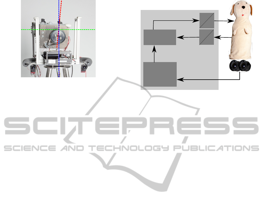
Figure 2: Interior of “Doggy” consisting of three revolute

joints. Their rotational axes intersect in one point leading to

redundancy. The bat, consisting of a sphere (Doggy’s head)

attached to a rod, is not shown.

dundancy should be intelligently used to distribute the

task to all joints. Moreover, the position, velocity and

time speciﬁcation is needed for a controlled play back

game and the robot has to comply to all three accu-

rately. We want a single controller fulﬁlling this task

of trajectory planning and intelligent distribution of

motor torques and joint angles to reach the goal po-

sition and velocity in time. Thus, we describe this

process as task level optimal control (TLOC).

Figure 3 shows the basic idea of the controllers

implementation on the system. As input parameters

the controller uses the actual state vector x consist-

ing of velocities and positions of motors and joints.

Moreover, it needs the goal parameters T , p and v

from a ball tracking algorithm to compute the optimal

policy. The policy is then combined with the state

vector and results to a torque control vector u. We

want to clarify that the detection of the goal parame-

ters as well as the tracking is not part of this paper.

1.3 Contribution

We combine trajectory planning and controlling in a

single controller using ﬁnite horizon optimal control.

The point we want to make in this paper, is that for

this task or similar tasks involving something to be

fulﬁlled at a given time, it is both elegant and practical

to formulate the task as an optimal control problem.

In particular the approach has the following beneﬁts:

• Automatic utilisation of redundancy

• Automatic generation of optimal motion

• Appropriate reaction on disturbances depending

on time (unlike trajectory planning plus position

control)

• Computation of an optimal (time dependent)

closed loop gain matrix (as opposed to an optimal

trajectory or optimal commands)

Optimal

Controller

Ball Tracking

and

Prediction

p, v, T

Figure 3: System overview of the controllers task bring-

ing the robots head in time T to a speciﬁed position p with

velocity v. The controller provides an optimal torque u to

fulﬁl this task. In Section 5.6 we will reconﬁgure this layout

to a chained implementation.

2 RELATED WORK

Most recently the motion planning described in

(Goretkin et al., 2013) is strongly related to our ap-

proach; although both have been independently devel-

oped. A ﬁnite time linear quadratic regulator (LQR)

is used together with RRT* to ﬁnd optimal solutions

to planning problems. We have in common the ﬁ-

nite horizon LQR, where the time is an additional in-

put parameter. The difference is that we provide an

independent feedback controller gain, whereas they

provide a trajectory to follow. The best trajectory is

found by iterate through all possible trajectories. This

is time consuming, which is neither applicable nor

necessary for the ball batting task as it does not in-

clude obstacles.

In (Perez et al., 2012) the feedback gain is com-

puted additionally to the cost matrix, but not explicitly

taken as controller gain. (Reist and Tedrake, 2010)

provides a control-policy look up table of feedback

stabilised trajectories, which all lead to the goal state,

by simulation-based LQR-Trees.

A lot of work concerning ball hitting tasks focuses

on learning strategies (Kober et al., 2010; Muelling

et al., 2013), where basic movements are learned by

teach in and later adapted to the situation, or are based

on trajectory planning in conjunction with a joint con-

troller to follow them as described in (Senoo et al.,

2006; Hu et al., 2010; Zhang and L, 2007; Nakai

et al., 1998).

Except for the volleyball robot of (Nakai et al.,

1998), all have the camera system separated from the

robot and they use industrial robots, which provide a

position interface, such that the focus is more on the

ICINCO2014-11thInternationalConferenceonInformaticsinControl,AutomationandRobotics

trajectory planning than on the controlling itself. The

volleyball robot is more designed as an entertainment

robot focusing on sport interaction playing balls back

to the opponent. But it is ﬁxed to a speciﬁc court in a

hall, which provides constant conditions leading to a

simpliﬁed controller.

The previous version of our robot (Laue et al.,

2013) is not ﬁxed to a dedicated environment and is

able to hit balls by moving to the predicted position,

but not with a speciﬁed velocity, so it can only inter-

cept and not play back.

In the following we describe the robot model with

its task space and limitations. Furthermore, we ex-

plain the dynamic programming procedure for the

optimal control process, followed by simulation ex-

periments. At the end we give a conclusion and an

overview about our future work.

3 MODEL

After giving an overview of the task, to rebound a ball

by controlling the EOF position such that it reaches

a goal position and velocity, we describe the model

of the robot our simulation and control algorithm is

based on. First rigid body kinematics and dynamics

are provided and later extended to the ﬂexible joint

case. We also mention the restrictions made.

3.1 Kinematics

The Kinematics describes the EOF position in 3D

world coordinates of the robot system using transla-

tion and rotation of each joint. Due to the intersecting

axes there is no translation between joints. Thus, the

position of the EOF is

kin

(q) = T

+ R

EOF

. (1)

Where q = (q

)

is the joint angle vector,

and T

EOF

are the translations from ﬁrst coordi-

nate system to world coordinates and EOF to third

coordinate system respectively. The rotations are

), R

) and R

) for ﬁrst, second and third

joint rotation. For our robot this results to

kin

(q) =





−s

)0.9m

+ s

)0.9m

0.9m +1 m





, (2)

where c

is cosq

, s

is sinq

, etc.

Having a sphere as bat, we can ignore the orienta-

tion of the end-effector.

Figure 4: “Doggy” kinematics and dynamics model with

coordinate systems, where red, green, blue is the x, y and z

coordinate respectively. The world coordinate system is on

the ground in the centre of the robot.

3.2 Dynamics

We derive the dynamics for our robot in two steps.

First we create the spatial vector notation (Feather-

stone, 2008; Featherstone, 2010), which we can plug

into the Matlab library Spatial v2 by (Featherstone,

2012). Therefore, we have to provide the connectiv-

ity graph, the geometry – which describes the trans-

lation and rotation, the joint type (revolute, prismatic,

helical) and the spatial inertia for each body.

We approximated the inertia matrices using sim-

ple geometry (Figure 4) and masses from a CAD

model. Most relevant for the controller is the bat mass

of 0.9 kg.

In the second step we obtain the equations of mo-

tion in the joint space form

M(q)

q +c(q,

q) +τ

(q) = τ

, (3)

where M(q), c(q,

q), τ

(q) and τ

are the joint space

inertia, Coriolis and centrifugal terms, gravitational

terms and motor torques respectively. The notation

for the joint angles, velocities and accelerations is q,

q and

q (Siciliano and Khatib, 2008).

To obtain the Coriolis and gravitational terms, we

use the inverse dynamics of the Spatial v2 library to-

gether with the symbolic toolbox of Matlab and set-

ting the acceleration

q to zero. The remaining joint

space inertia is provided by the composite-rigid-body

algorithm (Featherstone, 2010).

3.3 Elastic Joints

Our robot has relevant elasticities in the joints which

are mainly due to the tooth belt gear. Therefore,

we have to enhance the equation of motion (3) by

TaskLevelOptimalControlofaSimulatedBallBattingRobot

the elastic joint model, where motor angle, veloc-

ity and acceleration are described by θ

θ,

θ and

θ re-

spectively (Siciliano and Khatib, 2008; Spong, 1995;

Albu-Schaeffer et al., 2007).

The coupling between motor and joint is the tooth

belt, which can be approximated by a spring with

stiffness K and a damping D. In the following we

set the damping D to zero, which is the worst case.

M(q)

q +c(q,

q) +τ

(q) +K (q −θ

θ) = 0 (4)

θ +K (θ

θ −q) = τ

(5)

Where B and τ

are motor inertia and torque trans-

formed to the joint side with the gear ratio n

689

B = n

motor

, (6)

= n

motor

. (7)

We stack the dynamics into a nonlinear state space

representation

x = f

dyn

(x,u), deﬁning the state vector

x, the input vector u and the function f

dyn

(x,u) as

x =





, (8)

u = τ

, (9)

dyn

(x,u) =





−M(q)

−1

(

c(q,

q)+τ

(q)+K(q−θ

θ)

)

−B

−1

K(θ

θ−q)+B

−1





, (10)

which we use for our optimal control problem.

Not modeled. At the moment we ignore constraints

of joint angles and motor torques, as well as friction.

4 TASK LEVEL OPTIMAL

CONTROL

Having the robot model, kinematics of the EOF and

the equations of motion derived in the last section, we

now want to formulate our task of being at a desired

position with given speed in speciﬁed time, as a ﬁ-

nite horizon optimal control problem. The principle

will be explained at ﬁrst. Furthermore, we explain the

control parameters.

4.1 Finite Horizon Controller

The principle of a ﬁnite horizon controller is to min-

imise a cost function in the time interval [0, T ], by

ﬁnding an optimal policy, i. e. mapping from (x,t) 7→

u. The cost function consists of costs during the pro-

cess time, depending on state and command, and a

ﬁnal cost, where only the state contributes to the cost.

This is due to the ﬁnite time horizon, as the optimal

command in the last step is u = 0 and any other com-

mand would increase the cost. The general cost func-

tion is:

cost(x,u) = cost

(x(T )) +

cost(x(t), u(t))dt.

(11)

For our optimal control problem we deﬁne the ﬁ-

nal cost in dependency of the position p and the ve-

locity v. The process costs are then dependent on

the input torque and additionally on elastic vibrations

which are penalised.

cost(x,u) = cost

(x(T )) + cost

(x(T ))+

[cost

vib

(x(t)) + cost

(u(t))] dt

(12)

In the following the cost functions will be derived and

explained independently.

4.2 Cartesian Position

The position cost function formalises “be at position

p at time T ”. The Cartesian position of the EOF is

calculated by Equation (2). We deﬁne a new function

to penalise the quadratic deviation of actual system

position to a desired goal point p in world coordinates.

Hence, the position penalty is

cost

(x) = q

( f

kin

(q) −p)

, (13)

where q

is the penalisation parameter. The desired

point can have any value in 3D space, if it is not reach-

able by the EOF, the distance to it will be minimised.

4.3 Cartesian Velocity

The velocity cost function formalises “have velocity

v at time T ”. Considering our goal to reach a desired

position with a given velocity, we can apply a similar

penalisation as for the position to the velocity. Thus,

we need the derivative of the kinematics with respect

to time

vel

(q,

q) =

∂ f

kin

(q)

∂t

∂ f

kin

(q)

∂q

q. (14)

We construct the velocity penalty by penalising

the quadratic velocity difference from the desired ve-

locity v in Cartesian coordinates:

cost

(x) = q

( f

vel

(q,

q) −v)

. (15)

Only velocities in the tangential plane of the sphere’s

workspace can be achieved, for v outside that plane

the difference is minimised. Note, that because the

tangential plane depends on p, this will result in a

compromise between p and v and leading to an in-

crease of cost.

ICINCO2014-11thInternationalConferenceonInformaticsinControl,AutomationandRobotics

4.4 Vibration Reduction

The vibration reduction cost function formalises “os-

cillation is unwanted”. The ﬂexible joint system tends

to oscillate in the spring (q −θ

θ). We want the con-

troller to avoid this by penalising spring motion. So

cost

vib

(x) = q

vib



q −



(16)

is the overall vibration reduction penalisation.

4.5 Motor Torque

The motor torque cost function formalises “minimal

effort”. We deﬁne a cost function that penalises the

squared input torque by a factor r

. This is a canon-

ical choice of actuation costs, favours torques evenly

distributed over time and also corresponds to heat dis-

sipation of the DC-motor which we want to minimise.

cost

(u) = r

(17)

5 DYNAMIC PROGRAMMING

The previously deﬁned model and cost functions will

now be applied to compute the optimal control policy

expressed as a feedback gain matrix K

. Therefore,

we use dynamic programming to compute the optimal

control policy by backward induction. It starts with

the ﬁnal cost cost

= cost

(x(T )) + cost

(x(T )). For

each time-step T

it computes the effective cost of the

previous time-step as a function of that state x(T −T

)

by ﬁnding the x(T −T

) dependent optimal control

u(T −T

). This process goes back from x(T ) to x(0).

The case of dynamic programming we use here is

known as the ﬁnite horizon linear quadratic regulator

(Sontag, 1990). An advantage is the automatic com-

putation of the feedback gain matrix. Moreover, it is

a step by step method and can be easily adapted to

discrete systems with sample time T

controlled by an

LQR.

The LQR is based on a linear discrete system dy-

namics

n+1

= A

+ B

, (18)

= K

, (19)

where A and B denote the system and input matrix re-

spectively and n = t/T

is the discrete step time, which

is always an integer.

To integrate our system description derived in the

last sections into the dynamic programming algorithm

using a linear quadratic regulator, we ﬁrst have to lin-

earise our system and afterwards discretise it to match

into (18).

5.1 Linearisation

The equations of motion describe a nonlinear dy-

namic function f

dyn

(x,u). As mentioned the LQR is

working only on linear systems, we need to linearise

Equation (10). We do this by deriving the ﬁrst order

Taylor series around some linearisation point x

∗

and

∗

such that

lin

(x,u) = f

dyn

∗

) +

∂ f

dyn

∗

)

∂x

(x −x

∗

) +

∂ f

dyn

∗

)

∂u

(u −u

∗

)

(20)

is the linear system approximation. Determining the

linearisation points x

∗

and u

∗

will be discussed later.

As we can see in this Equation, we have a constant

term

c = f

dyn

∗

)−

∂ f

dyn

∗

)

∂x

∗

−

∂ f

dyn

∗

)

∂u

∗

(21)

which is not handled in (18). To make use of Equa-

tion (18), we can combine ﬁrst and zero order terms

into a single matrix. Thus, we get an afﬁne notation

(Goretkin et al., 2013), such that the resulting afﬁne

notation with

x = f

lin

(x,u) =

x +

Bu, (22)

will later ﬁt into (18) after discretisation, where

x =





and the matrices

A and

B are

A =



A c

0 0



∂ f

dyn

∗

)

∂x

0 0

, (23)

B =





∂ f

dyn

∗

)

∂u

. (24)

We apply the same process of linearisation to ob-

tain the costs. Thus we combine (13) and (15) to

cost

= cost

+ cost

such that we get the ﬁnal cost

cost

(x) =



(x,p,v)

z }| {

kin

(x)−p

vel

(x)−v





z}|{

I 0

0 q



kin

(x)−p

vel

(x)−v



, (25)

where I denotes the identity matrix.

Then we linearise f

(x,p,v) around x

∗

and ob-

tain



fpv





∂ f

∗

,p,v)

∂x

∗

,p,v) −

∂ f

∗

,p,v)

∂x

∗



(26)

and the linearised function

pvlin

(x,p,v) =

x. (27)

TaskLevelOptimalControlofaSimulatedBallBattingRobot

To get the ﬁnal cost in linearised form, we ﬁrst have

to build the square of Matrix

and penalise it by W

resulting to the penalisation matrix



fpv



. (28)

Finally, we have to multiply the ﬁnal penalisation ma-

trix

by the squared state afﬁne vector

x, giving us

the ﬁnal linearised cost

cost

ﬂin

(x) =

(T )

x(T ). (29)

For the vibration reduction cost we can do the

same linearisation as for the ﬁnal cost. Hence, we

have

cost

vib

(x) = (

vib

(x)

z}|{

q −

)

z}|{

vib

q −

). (30)

Linearising f

vib

(x) around x

∗

results in

J =



J c

vib





∂ f

vib

∗

)

∂x

vib

∗

) −

∂ f

vib

∗

)

∂x

∗



(31)

The vibration penalisation

Q in linearised form is then

Q =

J =



WJ J

vib

WJ c

vib



, (32)

which gives us the linearised vibration cost

cost

viblin

(x) =

(t)

x(t). (33)

For the torque cost in linearised form we can write

the result directly as a squared linear function of the

penalty. Thus, the cost is

cost

= u

(t)

z}|{

tau

I u(t), (34)

where R is the penalisation matrix of the input torque.

5.2 Discretisation

By now we have a linearisation of our continuous sys-

tem model. We now have to discretise it to ﬁt into

(18). The discretisation of a ﬁrst order differential

equation

z = Fz (35)

can be solved by using the approach

= e

, (36)

where T

is the sample time and e

is the matrix ex-

ponential (Berg et al., 2011). The result is the discrete

system

n+1

= F

. (37)

Adapting (37) with F =



0 0



and z =





and moreover using a ﬁrst order Taylor series approx-

imation for the matrix exponential we get the discrete

system



0 I



= I +FT

≈ e

, (38)

in the form of (18).

5.3 Feedback Gain

The computation of the feedback gain

can be done

recursively backward in time using dynamic program-

ming, as explained in (Sontag, 1990). Therefore, the

cost function

cost(x,u) =

N−1

∑

n=0

+ u

, (39)

is minimised leading to the algebraic discrete Riccati

Equation

Q +

n+1

−

n+1

(R +

n+1

)

−1

n+1

(40)

where

is set to

for the ﬁnal discrete step N =

T /T

. In the same iteration step we get the feedback

gain matrix

= −(R +

n+1

)

−1

n+1

. (41)

This is the core optimisation of the overall optimal

control algorithm.

5.4 Nonlinear Iterations

To solve the problem of hitting the ball at a speciﬁed

position with speciﬁed velocity at a speciﬁed time we

use nonlinear iterations. Thus, in the ﬁrst iteration

we compute an initial guess of our nonlinear system

(10) from the actual time-step n = 0 till the ﬁnal time-

step N. Based on this prediction the linearisations are

done and the feedback gains are provided for all fu-

ture steps. In the next iteration loop, the current sys-

tem state x(0) is used together with the linearisations

and feedback gains from the last step to predict the

behaviour for time-steps n = 1 to N and again lin-

earise the system based on this initial guess and pro-

viding the feedback gains. In each iteration the lin-

earised system converges more to the nonlinear sys-

tem. Moreover, if the linearised system diverges from

the nonlinear system, the next iteration update step

will tend the linearisation towards the nonlinear sys-

tem as the nonlinear current state x(0) is used as start

parameter. The cascaded implementation is explained

in Algorithm 1. The operating loop runs until the ball

has been hit. The most important steps are done in

systemForecast, lineariseFpv and dplqrAfﬁne.

In systemForecast we compute the linearised dis-

crete afﬁne system

and

in three steps.

First, we predict the system behaviour and lineari-

sation points x

∗

and u

∗

with (18) and (19) given

and

from the last iteration step. The lineari-

sation of the system is also done in systemForecast.

Hence, we create the ﬁrst order Taylor series in (21),

ICINCO2014-11thInternationalConferenceonInformaticsinControl,AutomationandRobotics

Algorithm 1: Cascaded implementation.

// Eq. (42)-(45)

1 [

∗

] =initialGuess(p,v,x(0));

2 for n

= [0,N −1] do

3 x(0) =getState();

4 if n

> 0 then

// Eq. (18), (19), (21), (23), (24), (38)

5 [

∗

] =systemForecast(

,x(0),

);

=lineariseFpv(x

∗

,p, v); // Eq. (26), (28)

7 end

// Eq. (40), (41)

=dplqrAfﬁne(

Q,R);

9 setGain(K

);

10 end

(23) and (24) using the provided linearisation points

to get the continuous system at those points. Finally,

we discretise the continuous system by (38).

Secondly, in the function lineariseFpv we obtain

the ﬁnal penalisation with x

∗

as linearisation point

of Equation (26). The resulting matrix

is then pe-

nalised by W

leading to the ﬁnal penalisation matrix

(Equation (28)).

Finally, the feedback gain for the controller is cal-

culated in dplqrAfﬁne based on the linearisations via

(40) and (41).

5.5 Initial Guess

Before iterating the loop of Algorithm 1 we need

to provide start conditions. This is fulﬁlled in ini-

tialGuess. As we have no actual control gains or sys-

tem linearisations at the iteration start, we need to pro-

vide a ﬁrst system prediction. Thus, we ﬁrst calculate

an initial guess for a desired ﬁnal state x

from p and

v which is then used to guess the intermediate states.

This is done by iterating the desired position and ap-

ply ﬁrst axis rotation R

) for different angles q

the range [−170

◦

,170

◦

] utilising 5

◦

steps. Obtaining

= T

+ R

(42)

as desired point in Axis 2 coordinates, except any ro-

tations of Coordinate System 2. Next we solve the

inverse kinematics for given q

invkin

,p) =















arctan





arcsin



√









(43)

This results in a set of possible angle rotations

reaching the same end-position p. Out of the set we

want to ﬁnd the one with the lowest overall rotation

Microcontroller

Computer

Task Level

Optimal

Control

Ball

Tracking

p, v, T

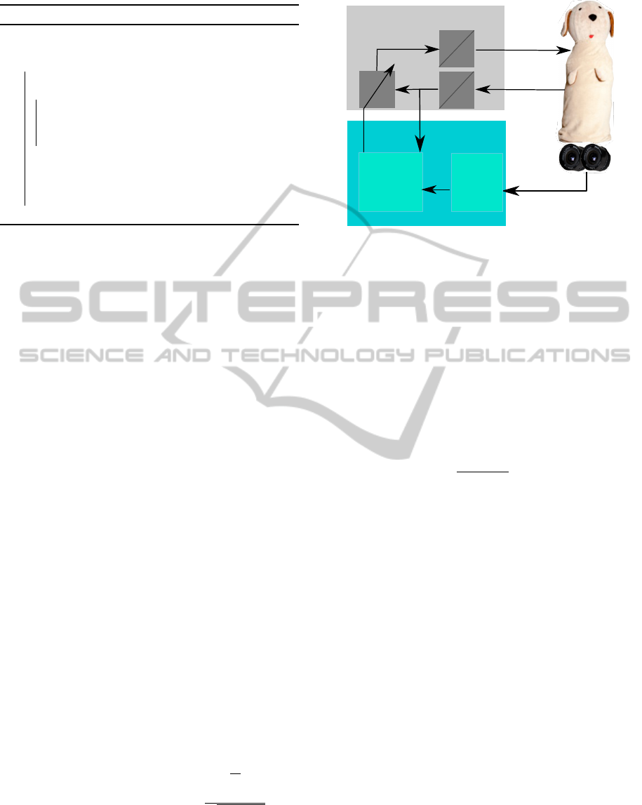
Figure 5: Distributed system with robot as plant, a micro-

controller as feedback controller and collector of sensor sig-

nals from the robot and a computer as ball detector, using

the cameras, and feedback gain optimiser.

of the joints, i. e.

= min

∑

(q(0) −q

invkin

,p))

, (44)

where q(0) is the current joint position.

For the angular velocity we plug q

into the Jaco-

bian of (14). Taking the pseudo-inverse, as the inverse

does not exist due to redundancy, results in the desired

velocity on the tangential plane



∂ f

kin

)

∂q



†

, (45)

where ()

†

denotes the pseudo-inverse.

To provide the discrete linearised system we as-

sume a straight line from current state x(0) to the ini-

tial desired state x

as linearisation points x

∗

. Though,

we suppose that the system will follow the states on

the line without any commanded torque (u

∗

= 0).

With these deﬁnitions we can compute the linearised

system by (21), (23) and (24) and descretise the result

by (38). Note, that this is just an initial guess which

has no inﬂuence to the ﬁnal optimal result as long as it

takes Algorithm 1 to the valley at the global optimum.

5.6 Chained Implementation

Computing a feedback gain instead of a trajectory al-

lows us to modify the system presented in the ﬁrst

section in Figure 3 to a faster distributed system in

Figure 5. Our described computations run separated

on a computer and microcontroller using discrete sig-

nals from camera and other sensors.

The microcontroller is responsible for the joints

torque control. It computes the torque using the feed-

back gain matrix

K and the actual system state x(0),

running on a sample time of 1ms.

TaskLevelOptimalControlofaSimulatedBallBattingRobot

Figure 5 also shows the camera system connected

to the computer which tracks throwing balls, which is

not part of this paper but basically explained in Sec-

tion 7. Moreover, velocity, position and time of im-

pact are predicted and provided and serve as our con-

trolling system goal parameters. The camera system

runs on a slower sample time of 50 ms. The slower

camera sample time is used as update time T

in the

loop of Algorithm 1. During each camera update one

iteration is processed. This allows us a forecast of the

states x

∗

, given the input u

∗

. The forecasted states are

then used as new linearisation points for the system at

the next camera update and a more precise calculation

of the controllers gain matrices

can be achieved.

The feedback gains are transferred after each iteration

to the microcontroller. This allows a faster sampling

time, as the microcontroller just computes one matrix

multiplication in each step. If it had to compute the

feedback gain matrix, such a fast sample time would

be impossible. Moreover, it allows a fast reaction on

disturbances in a linearised optimal way and later con-

verges to the nonlinear optimum by the iteration loop.

6 COMPARISON TO INFINITE

HORIZON LQR

Compared to the inﬁnite horizon LQR, which has no

ﬁnal time, we make use of the ﬁnite LQR by setting

the ﬁnal time as input parameter to the optimisation

problem. Moreover, the inﬁnite LQR would lead to a

fast achieving of the ﬁnal state, which causes greater

amount of input command. This is not useful with the

time horizon in mind, where we know when to reach

the ﬁnal state and so we are able to distribute the com-

manded torques more equally to each step. We will

show this in the next section by running a simulation

of our system and the distribution of a fast running

controller on a microcontroller and a slower running

feedback gain computation on a computer.

7 SYSTEM CONTEXT

In this paper we present the controller itself using the

position p, velocity v and the ﬁnal time T as input pa-

rameters for the controller. How to obtain these val-

ues is not part of this paper. However, for a better

understanding of the overall process we give a short

description about the system context. Throwing balls

towards the robot will lead to a detection of the balls

using two cameras mounted left and right from the

robots center axis. Circles are detected independently

in the left and right camera image. The detected

circles are then passed to either a Multiple Hypoth-

esis Tracker (MHT) that handles clutter and covers

missing detections followed by an Unscented Kalman

Filter (UKF) for estimation of position and veloc-

ity, which are used for prediction of the future states

(Laue et al., 2013). Alternatively they are passed to a

so called Fully Probabilistic Multiple Target Tracker

(FPMHT)(Birbach and Frese, 2013). With both algo-

rithms we intersect the predicted trajectory with the

workspace sphere and use the ﬁrst intersection as p.

This is implemented on the previous version of the

robot, with v ﬁxed to 0. The velocity needed for re-

turn is future work, but the theoretical implementation

has been investigated in (Hammer, 2011). Therefore,

a realistic rebound model of two balls can be used

to determine the direction vector and so the velocity

needed to rebound the ball.

8 SIMULATIONS

In a few scenarios we demonstrate the system be-

haviour using TLOC to reach a speciﬁed position and

velocity on different time constraints and we illus-

trate the robustness by applying a disturbance torque

to the system. All simulations are based on the

dataﬂow diagram of Figure 5 implemented in Matlab

and Simulink. There are three simulations combined:

A robot simulation, which runs with the forward dy-

namics of Spatial v2 library and some extensions for

the ﬂexible case; a microcontroller simulator, includ-

ing only the torque computation in each millisecond

and discretisation via sample and hold; the computer

simulator, for operating the TLOC every 50ms.

8.1 Elasticity Behaviour

First we illustrate the controller’s behaviour and sys-

tem reaction by reaching a deﬁned goal position p

with velocity v

at time T . Therefore, we set the pe-

nalisation for position q

, velocity q

, torque r

and

vibration reduction q

vib

. The values for the parame-

ters are shown in Table 1. Starting in upright position

p(0) with zero velocity v(0) we can see the behaviour

of the joints and the commanded torque in Figure 6.

We see the motor and joint positions and velocities

as well as the commanded torque. Due to the spring

stiffness K and the coupling between motor and joint

(q −θ

θ), we can see that the commanded torque acts

fast on the motor velocity, but the reaction of the joints

velocity is delayed. This delayed behaviour explains

the peaks in the commanded torque. At the ﬁrst lin-

earisation points the system does not react as the con-

ICINCO2014-11thInternationalConferenceonInformaticsinControl,AutomationandRobotics

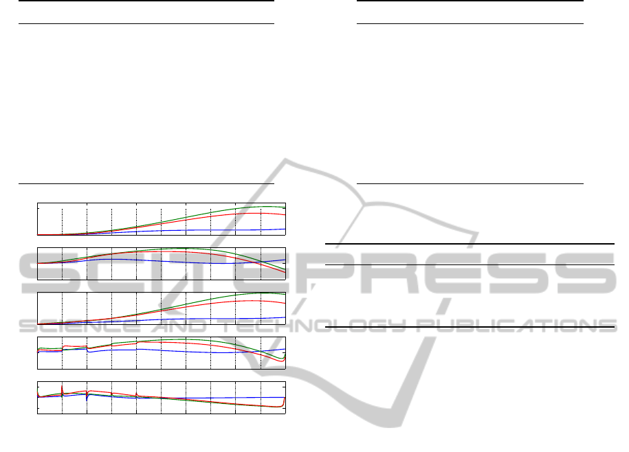
Table 1: Parameters for the elasticity behaviour.

Parameter Value

p(0) (0.0 0.0 1.9)

(0.45 0.636 1.45)

v(0) (0.0 0.0 0.0)

m/s

(0.0 −1.0 1.414)

m/s

T 0.5 s

5 ×10

−2

5 ×10

−2

vib

1.0 s

0.01 (Nm)

−2

0 100 200 300 400 500

◦

]

0 100 200 300 400 500

−200

200

˙q[

◦

/s]

0 100 200 300 400 500

θ[

◦

]

0 100 200 300 400 500

−200

200

θ[

◦

/s]

0 100 200 300 400 500

−10

u[Nm]

time[s/T

]

Figure 6: Reaching the goal position in T = 0.5s. Blue,

green, red denotes Axis 1, 2 and 3 respectively. Vertical

dashed lines denote the update times.

troller wanted due to linearisation errors, thus, to ful-

ﬁl a reaction on the joints position and velocity, the

spring has to be tensioned or loosened quickly. After

reaching the desired tension on the spring the torque

can be smoother.

Moreover, the torque is distributed over the whole

time span, bringing the axes to a position where the

goal could be reached. Here we accurately reach the

ﬁnal position p(T ) = (0.45 0.6359 1.4507)

m and

velocity v(T ) = (−0.0007 −1.0004 1.4121)

m/s

with the angular positions and velocities of Figure 6.

8.2 Time and Disturbance Behaviour

In this section we show the behaviour of the sys-

tem when the time horizon changes and if a torque

is added to the system as disturbance. Thus, we hit

the ball in every scenario in the same desired posi-

tion p

, with velocity v

and desired time T . Starting

in the upright EOF position p(0) with zero velocity

v(0). We set the penalisation for position q

, veloc-

Table 2: Parameters for the time and disturbance behaviour.

Parameter Value Unit

p(0) (0.0 0.0 1.9)

(0.0 0.0 1.9)

v(0) (0.0 0.0 0.0)

m/s

(5.0 0.0 0.0)

m/s

T 0.3 s

5.0 ×10

−2

5.0 ×10

−2

vib

1.0 s

0.01 (Nm)

−2

Table 3: Comparison of the experiments of reached position

and velocity to desired reference. Denoted in the table as

ref.

Position [mm] Velocity [m/s]

ref (0.0,0.0, 1900) (5.0,0.0, 0.0)

(a) (1.2,−0.1, 1900) (4.9989,−0.0001, −0.0067)

(b) (0.5,−0.1, 1900) (4.9996,−0.0001, −0.0029)

ity q

, torque r

and vibration reduction q

vib

and other

values as shown in Table 2.

The position and velocity results of our experi-

ments (a)–(c) are given in Table 3 . All ﬁgures includ-

ing the joint angle, joint velocity and the input com-

mand. Here we neglect the motor position and veloc-

ity in the ﬁgures as well as the vertical lines showing

the update. The update time has not changed and is

again 50ms.

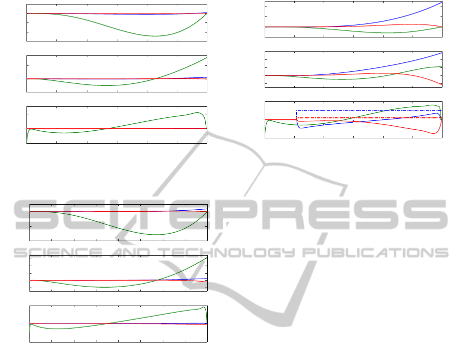
(a) We ﬁrst want to reach the desired position and

velocity in the given time of 0.3s as comparison ex-

ample. Therefore, Axis 2 turns backwards to accel-

erate the axis to the desired velocity (c. f. Figure 7).

Position and velocity are accurately reached.

(b) To show the time beneﬁt of the controller, we

change the desired time to T = 0.8s. This results in

a reduction in torque and “striking out” more from

the EOF rest position compared to the previous sim-

ulation (a). The further Axis 2 moves away from the

rest position the better it can accelerate the EOF by

less command torque. This is the result of giving the

controller more time to reach the goal, thus it can dis-

tribute the torque better over time (Figure 8).

by applying a disturbance torque such that the input

torque is τ

= u + τ

dist

. This can also be interpreted

TaskLevelOptimalControlofaSimulatedBallBattingRobot

0 50 100 150 200 250 300

−15

−10

−5

◦

]

0 50 100 150 200 250 300

−200

200

˙q[

◦

/s]

0 50 100 150 200 250 300

−20

u[Nm]

time[s/T

]

Figure 7: Simulation (a), reaching the goal position and ve-

locity in T = 0.3 s. Blue, green, red denotes Axis 1, 2 and 3

respectively.

0 100 200 300 400 500 600 700 800

−40

−20

◦

]

0 100 200 300 400 500 600 700 800

−100

100

200

300

˙q[

◦

/s]

0 100 200 300 400 500 600 700 800

−10

u[Nm]

time[s/T

]

Figure 8: Simulation (b), reaching the goal position and ve-

locity in T = 0.8 s. Blue, green, red denotes Axis 1, 2 and 3

respectively.

as a torque resulting from friction, which is demon-

strated later. A disturbance torque can be, e. g. some

external force pushing the head to another direction.

Figure 9 shows the disturbance as a step function of

dist

= (10 0 2)

Nm starting after 54 ms. Here you

can see the difference of forecast behaviour and real

behaviour by little spikes in the commanded torque at

the update steps. The reason is that the linearisation

points x

∗

are based on the modeled behaviour. When

the nonlinear system deviates from that behaviour, the

controller immediately reacts in a linearised optimal

way, because the output of dynamic programming is

not a sequence of torques but a policy, i. e. a sequence

of controller gains. In addition to this immediate lin-

earised response, in the next iteration of Algorithm 1

the measured state x(0) is used, linearisations are up-

dated and the policy is recomputed based on that state.

This results in a (close to) nonlinear optimal response

from that point on, visible in the small spike in u.

0 50 100 150 200 250 300

−20

◦

]

0 50 100 150 200 250 300

−200

200

400

600

˙q[

◦

/s]

0 50 100 150 200 250 300

−20

u[Nm]

time[s/T

]

Figure 9: Simulation (c). Reaching the goal position and

velocity in T = 0.3 s and applying a disturbance torque to

Axis 1 (dashed blue) and 3 (dashed red). Blue, green, red

denotes Axis 1, 2 and 3 respectively.

However, the goal position is met accurately (c. f.

Table 3) even if a disturbance is acting on the sys-

tem. Unlike trajectory optimisation followed by po-

sition control the system, however, does not hold its

trajectory (compare Figure 7 and 9) but ﬂexibly reacts

to the disturbances even distributing the motion in a

different way. The controller adapts to the new situ-

ation. Furthermore, the desired position and velocity

are hold accurately, which would not be the case if

a joint torque trajectory would have been set to the

system.

8.3 Friction

In this simulation we want to show how the con-

troller deals with friction, which is unconsidered in

the model but added to the plant. The goal position

and velocity is given in Table 3. We set the static

friction to 5 Nm and the Coulomb friction to 4 Nm.

As friction is a non-differentiable function, which is

a problem for the simulation solver, we approximate

the friction by a sigmoid function to get a soft transi-

tion when the velocity is around zero. In this exper-

iment we let the friction act on the motor side, such

that a zero crossing of the input torque u leads to a

change in the motor acceleration

θ. If the resulting

velocity changes its direction, it can be seen in the

friction too. If the velocity is around zero, then fric-

tion is between minimum and maximum static friction

(c. f. Figure 10 the red and blue dashed lines). Com-

pared to the real world we differ in the correctness of

the friction model, but we are interested in moving,

so we do not need to be accurate when the friction

is highest, which is at zero velocity. Moreover, we

reached the position (1.0,0.0,1900) [mm] and veloc-

ity (4.9982,0.0006,−0.0056) [m/s] accurately, which

ICINCO2014-11thInternationalConferenceonInformaticsinControl,AutomationandRobotics

0 50 100 150 200 250 300

−20

−10

◦

]

0 50 100 150 200 250 300

−200

200

400

˙q[

◦

/s]

−50

u[Nm]

0 50 100 150 200 250 300

−5

[Nm]

time[s/T

]

Figure 10: Reaching the goal position and velocity in T =

0.3s and applying friction to all axes (dashed). Blue, green,

red denotes Axis 1, 2 and 3 respectively.

shows the robustness also against friction which is not

considered in the model.

8.4 Deviation of Model Parameters

In the previous tests we expected that the model of

the plant and the plant itself are identically. In this

simulation we identify how the controller is acting, if

the plant parameters are varied, i. e. varying the val-

ues for motor inertia B, joint spring stiffness K and

damping D. First, we run the simulations 100 times

and change the parameters B and K in the range of

±10% of the modeled value. Secondly, we repeat the

test and additionally vary the damping D coefﬁcient

within [0,K ·0.1s].

Figure 11 points out, that a divergence of the pa-

rameters will lead to a deviation of the accuracy. The

damping parameter seems more critical (+ markers),

but the error still be below 2.5cm, which is precise

enough to hit the ball despite considerabel velocity

error.

8.5 Example of Intended Use

Finally, we provide a video

where four motion se-

quences are shown. Each sequence consists of a

movement reaching a desired position with given ve-

locity at a speciﬁed time and moving back to the rest

upright position with velocity zero. Then the next se-

quence starts. This simulates the ball batting task.

In such a task the robot waits for thrown balls in

its initial position, then accelerates towards the balls

intersection point. Hitting the ball with desired veloc-

http://www.informatik.uni-

bremen.de/agebv2/downloads/videos/schuethe icinco 14 doggyExampleMotion.mp4

0 0.005 0.01 0.015 0.02 0.025

0.05

0.1

0.15

0.2

0.25

0.3

0.35

kv − v

kp − p

Figure 11: Euclidean distance from reached position and

velocity to desired one with varied parameters B and K

within ±10%(x markers) and additionally with D (+ mark-

ers).

ity should return the ball to the player thrown the ball

or towards another person standing next to the robot.

The video just simulates the robot motion and po-

sition. The speciﬁed position is a ball and the desired

velocity is marked as an arrow. The arrow direction

shows the desired Cartesian velocity direction. If the

desired velocity is set to zero, no arrow will be drawn.

It is shown that the movements include all axes.

Moreover, the dynamic of the robot can be seen. It

shows fast and slow movements, depending on the de-

sired time for a movement and the speciﬁed velocity.

9 CONCLUSION AND FUTURE

WORK

We have shown an optimal state feedback controller

for a simulated, redundant and ﬂexible robot. The

controller is capable of steering the joints position and

velocity such that they are reaching a desired Carte-

sian position under and velocity at a given time, which

is needed to rebound a ball. Moreover, the controller

intelligently distributes the torques to all axes by mak-

ing use of the redundancy and hence, having less max-

imum torque for a single axis. Additionally, we see an

adaption of the controller to changing conditions.

The presented controller will be extended by con-

straints on joint angles and motor torques - which

were neglected in this paper -, to adapt our approach

more to the physical system. Furthermore, we have

to take friction into consideration, which is challeng-

ing in slow joint movements, but we have shown that

the controller can handle it without knowing the fric-

tion. Finally, the whole process has to be imple-

mented on the real robot, including system identiﬁ-

TaskLevelOptimalControlofaSimulatedBallBattingRobot

cation and state estimation, to verify our simulated

results. For playing back balls accurately we have to

calibrate the system to get a good ﬁtting model. A

very worthwhile further extension could be to include

the physics of playing back the ball into the optimisa-

tion, so the system does not try to achieve a position

and velocity as explained herein, it would optimise

the ball’s goal position, e. g. an opponent player’s po-

sition or any other desired position surrounding the

robot.

ACKNOWLEDGEMENTS

This work has been supported by the Graduate School

SyDe, funded by the German Excellence Initiative

within the University of Bremen’s institutional strat-

egy.

REFERENCES

Albu-Schaeffer, A., Ott, C., and Hirzinger, G. (2007). A

uniﬁed passivity-based control framework for posi-

tion, torque and impedance control of ﬂexible joint

robots. The International Journal of Robotics Re-

search, 26(1):23–39.

Berg, J., Patil, S., Alterovitz, R., Abbeel, P., and Goldberg,

K. (2011). LQG-based planning, sensing, and control

of steerable needles. In Hsu, D., Isler, V., Latombe,

J.-C., and Lin, M., editors, Algorithmic Foundations

of Robotics IX, volume 68 of Springer Tracts in Ad-

vanced Robotics, pages 373–389. Springer Berlin Hei-

delberg.

Birbach, O. and Frese, U. (2013). A precise tracking algo-

rithm based on raw detector responses and a physical

motion model. In Proceedings of the IEEE Interna-

tional Conference on Robotics and Automation (ICRA

2013), Karlsruhe, Germany, pages 4746–4751.

Featherstone, R. (2008). Rigid body dynamics algorithms,

volume 49. Springer Berlin.

Featherstone, R. (2010). A beginner’s guide to 6-D vec-

tors (part 2) [tutorial]. Robotics Automation Maga-

zine, IEEE, 17(4):88–99.

Featherstone, R. (2012). Spatial v2 (version 2).

http://royfeatherstone.org/spatial/v2/notice.html.

Goretkin, G., Perez, A., Platt, R., and Konidaris, G. (2013).

Optimal sampling-based planning for linear-quadratic

kinodynamic systems. In Robotics and Automa-

tion (ICRA), 2013 IEEE International Conference on,

pages 2429–2436.

Hammer, T. (2011). Aufbau, Ansteuerung und Simulation

eines interaktiven Ballspielroboters. Master’s thesis,

Universitaet Bremen.

Hu, J.-S., Chien, M.-C., Chang, Y.-J., Su, S.-H., and Kai,

C.-Y. (2010). A ball-throwing robot with visual feed-

back. In Intelligent Robots and Systems (IROS), 2010

IEEE/RSJ International Conference on, pages 2511–

2512.

Kober, J., Mulling, K., Kromer, O., Lampert, C. H.,

Scholkopf, B., and Peters, J. (2010). Movement tem-

plates for learning of hitting and batting. In Robotics

and Automation (ICRA), 2010 IEEE International

Conference on, pages 853–858.

Laue, T., Birbach, O., Hammer, T., and Frese, U. (2013). An

entertainment robot for playing interactive ball games.

In RoboCup 2013: Robot Soccer World Cup XVII,

Lecture Notes in Artiﬁcial Intelligence. Springer. to

appear.

Muelling, K., Kober, J., Kroemer, O., and Peters, J. (2013).

Learning to select and generalize striking movements

in robot table tennis. The International Journal of

Robotics Research, 32(3):263–279.

Nakai, H., Taniguchi, Y., Uenohara, M., Yoshimi, T.,

Ogawa, H., Ozaki, F., Oaki, J., Sato, H., Asari, Y.,

Maeda, K., Banba, H., Okada, T., Tatsuno, K., Tanaka,

E., Yamaguchi, O., and Tachimori, M. (1998). A vol-

leyball playing robot. In Robotics and Automation,

1998. Proceedings. 1998 IEEE International Confer-

ence on, volume 2, pages 1083–1089 vol.2.

Perez, A., Platt, R., Konidaris, G., Kaelbling, L., and

Lozano-Perez, T. (2012). LQR-RRT*: Optimal

sampling-based motion planning with automatically

derived extension heuristics. In Robotics and Automa-

tion (ICRA), 2012 IEEE International Conference on,

pages 2537–2542.

Reist, P. and Tedrake, R. (2010). Simulation-based lqr-

trees with input and state constraints. In Robotics and

Automation (ICRA), 2010 IEEE International Confer-

ence on, pages 5504–5510.

Senoo, T., Namiki, A., and Ishikawa, M. (2006). Ball con-

trol in high-speed batting motion using hybrid trajec-

tory generator. In Robotics and Automation, 2006.

ICRA 2006. Proceedings 2006 IEEE International

Conference on, pages 1762–1767.

Siciliano, B. and Khatib, O. (2008). Springer handbook of

robotics. Springer.

Sontag, E. D. (1990). Mathematical control theory: deter-

ministic ﬁnite dimensional systems. Texts in applied

mathematics ; 6. Springer, New York [u.a.].

Spong, M. W. (1995). Adaptive control of ﬂexible joint

manipulators: Comments on two papers. Automatica,

31(4):585 – 590.

Zhang, P.-Y. and L, T.-S. (2007). Real-time motion plan-

ning for a volleyball robot task based on a multi-agent

technique. Journal of Intelligent and Robotic Systems,

49(4):355–366.

ICINCO2014-11thInternationalConferenceonInformaticsinControl,AutomationandRobotics